Welcome to the slopes vignette, a type of long-form
documentation/article that introduces the core functions and
functionality of the slopes package.
Installation
You can install the released version of slopes from CRAN with:
install.packages("slopes")Install the development version from GitHub with:
# install.packages("remotes")
remotes::install_github("ropensci/slopes")
Installation for DEM downloads
If you do not already have DEM data and want to make use of the
package’s ability to download them using the ceramic
package, install the package with suggested dependencies, as
follows:
# install.packages("remotes")
remotes::install_github("ropensci/slopes", dependencies = "Suggests")
Furthermore, you will need to add a MapBox API key to be able to get
DEM datasets, by signing up and registering for a key at
https://account.mapbox.com/access-tokens/ and then
following these steps:
usethis::edit_r_environ()
# Then add the following line to the file that opens:
# MAPBOX_API_KEY=xxxxx # replace XXX with your api key
Functions
Elevation
-
elevation_add()Take a linestring and add a third dimension (z) to its coordinates -
elevation_get()Get elevation data from hosted maptile services (returns aSpatRaster) -
elevation_extract()Extract elevations from coordinates
Slope calculation
-
slope_vector()Calculate the gradient of line segments from distance and elevation vectors -
slope_distance()Calculate the slopes associated with consecutive distances and elevations -
slope_distance_mean()Calculate the mean average slopes associated with consecutive distances and elevations -
slope_distance_weighted()Calculate the slopes associated with consecutive distances and elevations, weighted by distance -
slope_matrix()Calculate the slope of lines based on a DEM matrix -
slope_matrix_mean()Calculate the mean slope of lines based on a DEM matrix -
slope_matrix_weighted()Calculate the weighted mean slope of lines based on a DEM matrix -
slope_raster()Calculate the slope of lines based on a raster DEM -
slope_xyz()Calculate the slope of lines based on XYZ coordinates
Plotting
-
plot_slope()Plot slope data for a 3d linestring
Helper functions
-
sequential_dist()Calculate cumulative distances along a linestring -
z_value()Extract Z coordinates from ansfcobject -
z_start()Get the starting Z coordinate -
z_end()Get the ending Z coordinate -
z_mean()Calculate the mean Z coordinate -
z_max()Get the maximum Z coordinate -
z_min()Get the minimum Z coordinate -
z_elevation_change_start_end()Calculate the elevation change from start to end -
z_direction()Determine the direction of slope (uphill/downhill) -
z_cumulative_difference()Calculate the cumulative elevation difference
Examples
This section shows some basic examples of how to use the
slopes package.
First, load the necessary packages and data:
library(slopes)
library(sf)
#> Linking to GEOS 3.12.2, GDAL 3.8.4, PROJ 9.4.0; sf_use_s2() is TRUE
#> WARNING: different compile-time and runtime versions for GEOS found:
#> Linked against: 3.12.2-CAPI-1.18.2 compiled against: 3.12.1-CAPI-1.18.1
#> It is probably a good idea to reinstall sf (and maybe lwgeom too)

# Load example data
data(lisbon_route)
dem_lisbon <- dem_lisbon()
Add elevation to a linestring
If you have a 2D linestring and a DEM, you can add elevation data to
the linestring using elevation_add():
sf_linestring_xyz_local <- elevation_add(lisbon_route, dem = dem_lisbon)
head(sf::st_coordinates(sf_linestring_xyz_local))
#>              X         Y        Z L1
#> [1,] -88202.31 -105757.6 55.91552  1
#> [2,] -88201.67 -105762.3 55.52176  1
#> [3,] -88200.54 -105770.5 54.62495  1
#> [4,] -88199.42 -105778.7 50.82914  1
#> [5,] -88198.29 -105786.9 50.76749  1
#> [6,] -88205.89 -105786.3 49.22162  1
If you don’t have a local DEM, elevation_add() can
download elevation data (this requires a MapBox API key and the
ceramic package):
# Requires a MapBox API key and the ceramic package
# sf_linestring_xyz_mapbox = elevation_add(lisbon_route)
# head(sf::st_coordinates(sf_linestring_xyz_mapbox))
Calculate slope
Once you have a 3D linestring (with XYZ coordinates), you can
calculate its average slope using slope_xyz():
slope <- slope_xyz(sf_linestring_xyz_local)
slope
#>          1
#> 0.07817098
Plot elevation profile
You can visualize the elevation profile of a 3D linestring using
plot_slope():
# ensure a palette and breaks exist
brks <- c(3, 6, 10, 20, 40, 100)
pal <- slopes_palette(length(brks) - 1)

plot_slope(sf_linestring_xyz_local, pal = pal, brks = brks)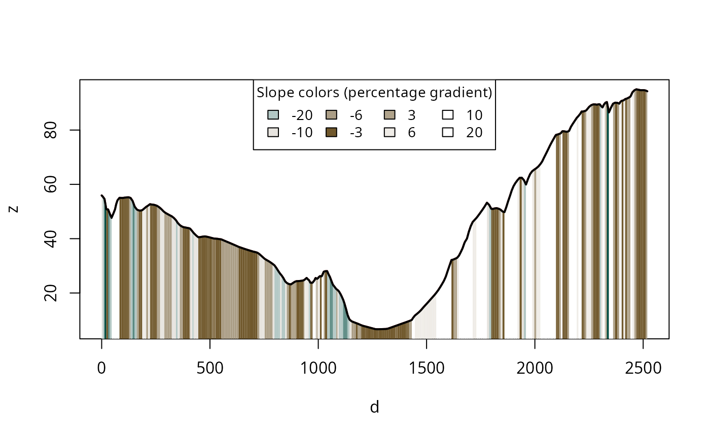
Working with segments
The slopes package can also work with individual
segments of a linestring. There are two ways to split a route into
segments:
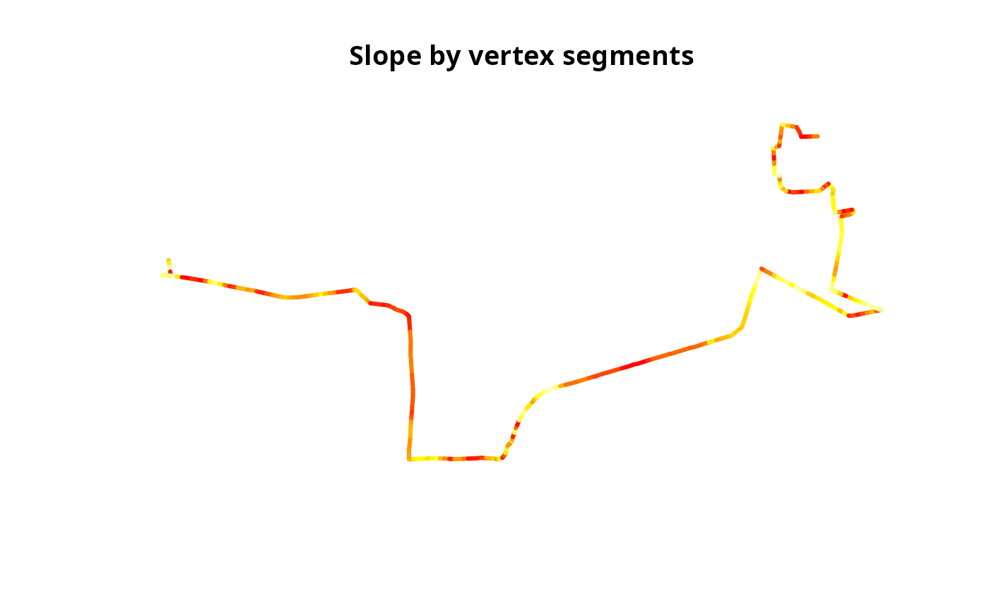
By vertex (native segments of the linestring)
route_to_segments() splits the route at every existing
vertex, producing one 2-point segment per coordinate pair:
lisbon_route_xyz <- elevation_add(lisbon_route, dem = dem_lisbon())
lisbon_route_segments_xyz <- route_to_segments(lisbon_route_xyz)
lisbon_route_segments_xyz$slope <- slope_xyz(lisbon_route_segments_xyz)
summary(lisbon_route_segments_xyz$slope)
#>      Min.   1st Qu.    Median      Mean   3rd Qu.      Max.       NAs
#> 0.0001026 0.0239350 0.0545492 0.0770948 0.1076403 0.4570354        24
plot(st_geometry(lisbon_route_segments_xyz),
  col = heat.colors(length(lisbon_route_segments_xyz$slope))[rank(lisbon_route_segments_xyz$slope)],
  lwd = 3, main = "Slope by vertex segments"
)
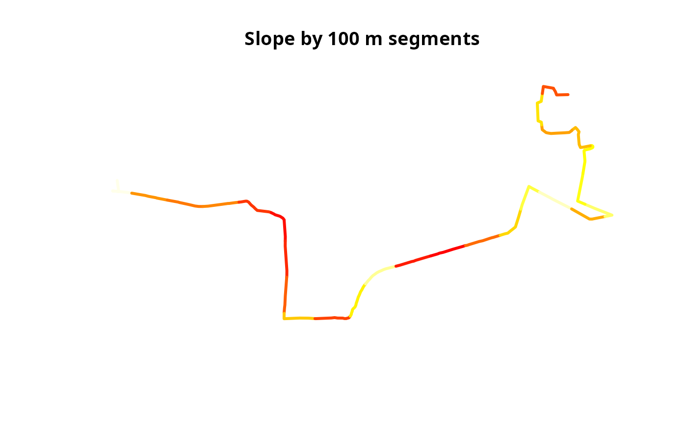
By fixed length (using stplanr)
stplanr::line_segment() splits the route into segments
of a given length (e.g. 100 m). Elevation must be added after
segmenting, since the new endpoints won’t have Z coordinates yet:
lisbon_route_100m <- stplanr::line_segment(lisbon_route, segment_length = 100)
lisbon_route_100m_xyz <- elevation_add(lisbon_route_100m, dem = dem_lisbon())
lisbon_route_100m_xyz$slope <- slope_xyz(lisbon_route_100m_xyz)
summary(lisbon_route_100m_xyz$slope)
#>    Min. 1st Qu.  Median    Mean 3rd Qu.    Max.
#> 0.01366 0.04364 0.06697 0.07822 0.11096 0.16180
plot(st_geometry(lisbon_route_100m_xyz),
  col = heat.colors(length(lisbon_route_100m_xyz$slope))[rank(lisbon_route_100m_xyz$slope)],
  lwd = 3, main = "Slope by 100 m segments"
)
This vignette provides a basic overview. For more detailed information and advanced use cases, please refer to the other vignettes and the function documentation.