Introduction
Although there are several ways to name “slope”, such as “steepness”,
“hilliness”, “inclination”, “aspect”, “gradient”, “declivity”, the
referred slopes in this package can be defined as the
“longitudinal gradient” of linear geographic entities, as defined in the
context of rivers by(Cohen et al.
2018).
The package was initially developed to research road slopes to support evidence-based sustainable transport policies. Accounting for gradient when planning for new cycling infrastructure and road space reallocation for walking and cycling can improve outcomes, for example by helping to identify routes that avoid steep hills. The package can be used to calculate and visualise slopes of rivers and trajectories representing movement on roads of the type published as open data by Ariza-López et al. (2019).
Data on slopes are useful in many fields of research, including hydrology, natural hazards (including flooding and landslide risk management), recreational and competitive sports such as cycling, hiking, and skiing. Slopes are also also important in some branches of transport and emissions modelling and ecology. A growing number of people working with geospatial data require accurate estimates of gradient, including:
- Transport planning practitioners who require accurate estimates of roadway gradient for estimating energy consumption, safety and mode shift potential in hilly cities (such as Lisbon, the case study city used in the examples in the documentation).
- Vehicle routing software developers, who need to build systems are sensitive to going up or down steep hills (e.g. bicycles, trains, and large trucks), such as active travel planning, logistics, and emergency services.
- Natural hazard researchers and risk assessors require estimates of linear gradient to inform safety and mitigation plans associated with project on hilly terrain.
- Aquatic ecologists, flooding researchers and others, who could benefit from estimates of river gradient to support modelling of storm hydrographs
There likely other domains where slopes could be useful, such as agriculture, geology, and civil engineering.
An example of the demand for data provided by the package is a map
showing gradients across Sao Paulo (Brazil, see image below) that has
received more than 200 ‘likes’ on Twitter and generated conversations:
https://twitter.com/DanielGuth/status/1347270685161304069
Calculating slopes
The most common slope calculation method is defined by the vertical difference of the final and start point or line height (z1 and z0) divided by the horizontal length that separates them.
Depending on the purpose of application, it might me relevant to understand how hilliness is estimated.

Measures of route hilliness
There are many ways to measure hilliness, mean distance weighted hilliness being perhaps the most common. These measures, and their implementation (or current lack thereof) in the package is summarised below.
Mean distance weighted gradient. Perhaps the simplest and most widely applicable measure is the mean gradient of the route. This should be weighted by the distance of each segment. Implemented by default in the
slope_raster()function.Max gradient. For activities like cycling, where steep hills have a disproportionate impact, it may be useful to consider the maximum gradient. Not yet implemented.
Xth percentile gradient. Since the maximum gradient gives no information about the rest of the route segments, other measures such as the 75th percentile gradient could be more informative. Not yet implemented.
Inverted harmonic mean. If we use the following formula we will get an index that (like the arithmetic mean) makes use of the full dataset, but that is weighted towards the higher gradient segments. Whether this index, the formula of which is shown below, is helpful, remains to be tested. Not yet implemented.
Segments in a route: Cumulative slope
The length of a segment in a route is also a relevant factor to have in consideration. If it is ok to bike through a segment of 8% with xx length, it is not so ok to bike in four segments in a row like that one (8% for 4xx length), as illustrated bellow.
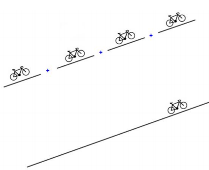
Illustration of the importance of slope length. 4 segments with an 8% gradient is not the same as a single segment with a gradient of 8%.
This is accounted for in slope calculation methods that take the distance-weighted mean of slopes.
x = c(0, 2, 3, 4, 5, 9)
y = c(0, 0, 0, 0, 0, 9)
z = c(1, 2, 2, 4, 3, 1) / 10
m = cbind(x, y, z)
d = sequential_dist(m = m, lonlat = FALSE)

slopes::slope_distance_weighted(d = d, elevations = z)
#> [1] 0.04040715
slopes::slope_distance_mean(d = d, elevations = z)
#> [1] 0.07406138
The slope estimate that results from the distance-weighted mean is lower than the simple mean. This is common: steep slopes tend to be short!
A graphical representation of the scenario demonstrated above is shown in Figure @ref(fig:weighted), that shows the relatively long and flat final segment reduces the slope by half.
plot(x, z, ylim = c(-0.5, 0.5), type = "l")
(gxy = slope_matrix(m, lonlat = FALSE))
#> [1]  0.05000000  0.00000000  0.20000000 -0.10000000 -0.02030692
abline(h = 0, lty = 2)
points(x[-length(x)], gxy, col = "blue")
title("Distance elevation profile",
  sub = "Points show calculated gradients of subsequent lines")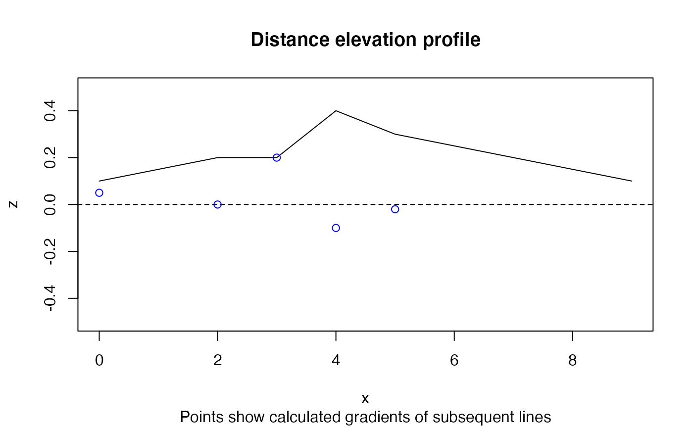
Illustration of example data that demonstrates distance-weighted mean gradient, used by default in the slopes package.