Getting Started with Athlytics

Welcome to Athlytics

This tutorial will guide you through a complete workflow—from loading your Strava data to generating training analytics. By the end, you’ll understand how to use all core features of Athlytics for longitudinal exercise physiology analysis.

What You’ll Learn:

How to load and explore your Strava export data
Calculate and interpret training load metrics (ACWR)
Analyze aerobic fitness trends (Efficiency Factor)
Quantify cardiovascular drift (Decoupling)
Track personal bests and performance progression
Export results for further analysis

Time Required: 30-60 minutes

Prerequisites

Installation

For installation instructions, see the README. The quick version:

# CRAN (stable)
install.packages("Athlytics")

# GitHub (latest features)
remotes::install_github("HzaCode/Athlytics")

Your Strava Data Export

You’ll need a Strava data export ZIP file. If you haven’t exported your data yet, start from Strava and follow the steps in the README Quick Start.

Quick Summary: 1. Set Strava language to English first: Strava Settings → Display Preferences → Language → English. The CSV export uses localized column headers, so non-English exports will fail to parse correctly. 2. Go to Strava Settings → My Account → Download or Delete Your Account 3. Request “Download” (NOT delete!) 4. Wait for email with download link 5. Download the ZIP file (e.g., export_12345678.zip) 6. Don’t unzip it — Athlytics reads ZIP files directly

Loading Your Data

Basic Loading

library(Athlytics)
library(dplyr) # For data manipulation

# Load your activities
activities <- load_local_activities("path/to/export_12345678.zip")

# View the first few rows
head(activities)

Understanding the Data Structure

Let’s explore what we just loaded:

# How many activities do you have?
nrow(activities)
# Example output: [1] 847

# What sports are in your data?
table(activities$type)
# Example output:
#   Ride  Run  Swim
#    312  498    37

# Date range
range(activities$date, na.rm = TRUE)
# Example output: [1] "2018-01-05" "2024-12-20"

# Key columns in the dataset
names(activities)

Important Columns:

id — Unique activity identifier
date — Activity date
type — Activity type (Run, Ride, Swim, etc.)
distance — Distance in kilometers
moving_time — Moving time in seconds
average_heartrate — Average heart rate (if recorded)
max_heartrate — Maximum heart rate
average_speed — Average speed (m/s)
average_watts — Average power for cycling (if available)
elevation_gain — Total elevation gain (meters)

Data Quality Checks

Before analysis, it’s good practice to check your data:

# Summary statistics
summary(activities |> select(distance, moving_time, average_heartrate))

# Check for missing heart rate data
sum(!is.na(activities$average_heartrate)) / nrow(activities) * 100
# Shows % of activities with HR data

# Activities without HR data
activities |>
  filter(is.na(average_heartrate)) |>
  count(type)

Pro Tip: Many Athlytics functions require heart rate data. Filter for !is.na(average_heartrate) when calculating EF or decoupling.

Filtering Your Data

For focused analysis, you’ll often want to filter by type or date:

# Only running activities
runs <- activities |>
  filter(type == "Run")

# Recent activities (last 6 months)
recent <- activities |>
  filter(date >= Sys.Date() - 180)

# Runs with heart rate data from 2024
runs_2024_hr <- activities |>
  filter(
    type == "Run",
    !is.na(average_heartrate),
    lubridate::year(date) == 2024
  )

# Long runs only (> 15 km)
long_runs <- activities |>
  filter(type == "Run", distance > 15)

Core Analyses

Now let’s dive into the main analytical features. Each metric provides different insights into your training and physiology.

1. Training Load (ACWR)

What is ACWR?

The Acute:Chronic Workload Ratio (ACWR) compares your recent training (acute load, typically 7 days) to your long-term baseline (chronic load, typically 28 days). It helps you monitor whether you are ramping up training too quickly.

Basic ACWR Calculation

# Calculate ACWR for all running activities
acwr_data <- calculate_acwr(
  activities_data = runs,
  activity_type = "Run", # Filter by activity type
  load_metric = "duration_mins", # Can also be "distance_km" or "hrss"
  acute_period = 7, # 7-day rolling average
  chronic_period = 28 # 28-day rolling average
)

# View results
head(acwr_data)

Output Columns:

date — Date
atl — Acute Training Load (7-day rolling average)
ctl — Chronic Training Load (28-day rolling average)
acwr — Raw ACWR ratio (ATL / CTL)
acwr_smooth — Smoothed ACWR (rolling mean of acwr)

Visualizing ACWR

# Basic plot
plot_acwr(acwr_data)

# With risk zones highlighted (recommended)
plot_acwr(acwr_data, highlight_zones = TRUE)

Demo with Sample Data:

# Load built-in sample data
data("sample_acwr", package = "Athlytics")

# Plot ACWR with risk zones
plot_acwr(sample_acwr, highlight_zones = TRUE)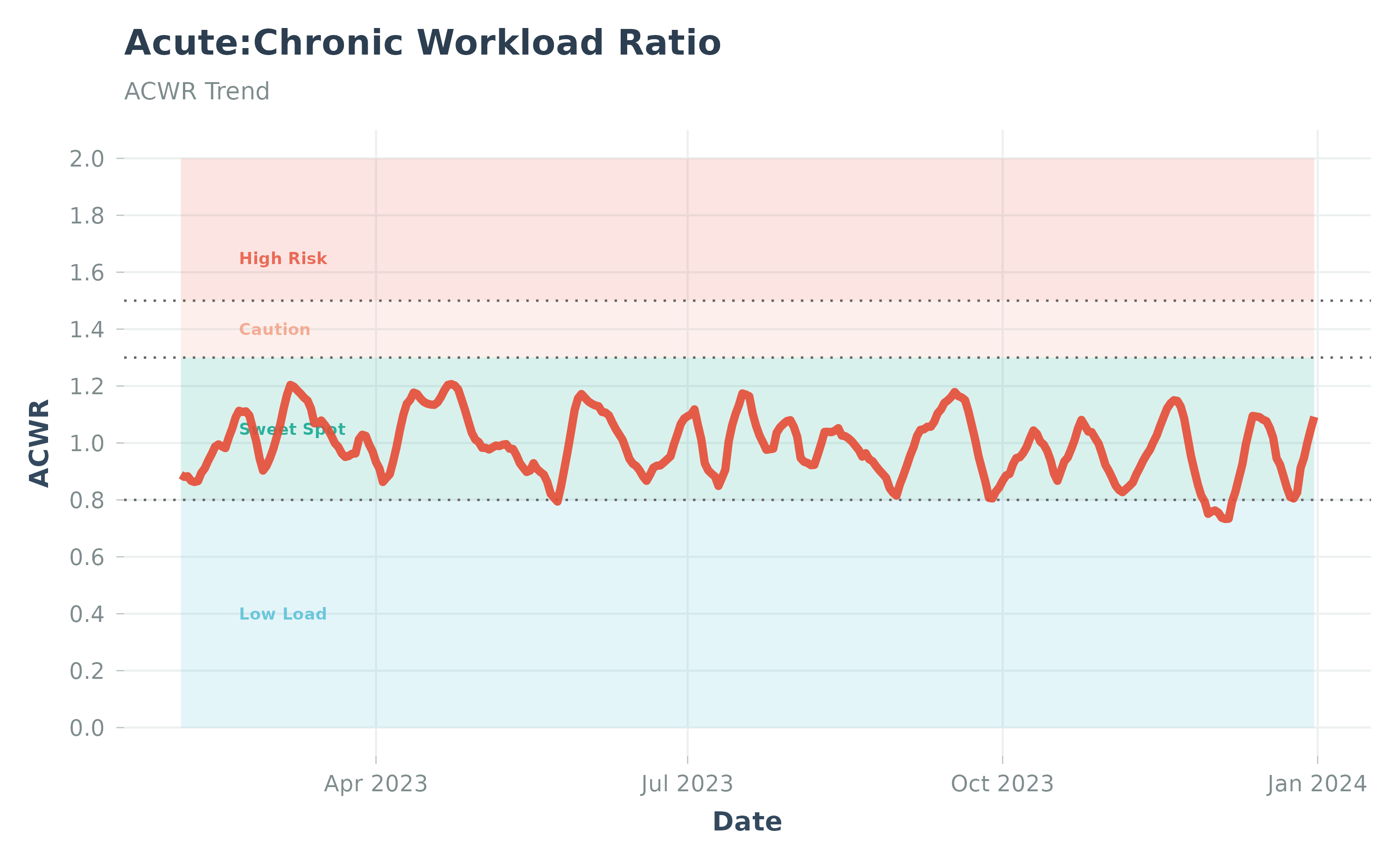

ACWR visualization using sample data

Risk Zones

< 0.8 — Undertraining (fitness may decline)
0.8-1.3 — “Sweet spot” (optimal adaptation zone)
1.3-1.5 — Moderate risk (load increasing rapidly)
> 1.5 — High risk (excessive load spike, injury risk)

Interpreting Your ACWR

What to look for:

Gradual increases = Good progressive overload
Sharp spikes above 1.5 = Warning signs, consider recovery
Extended periods < 0.8 = May need to increase training volume
Stable values in 0.8-1.3 = Optimal training stimulus

Practical Example:

# Identify high-risk periods
high_risk <- acwr_data |>
  filter(acwr_smooth > 1.5) |>
  select(date, atl, ctl, acwr_smooth)

print(high_risk)

# Check recent trend
recent_acwr <- acwr_data |>
  filter(date >= Sys.Date() - 60) |>
  arrange(desc(date))

head(recent_acwr, 10)

Choosing Load Metrics

Different load metrics for different goals:

duration_mins — Simple, works for all sports, good for general monitoring
distance_km — Better for distance-focused training (marathon prep)
hrss — Most accurate for physiological load (requires HR data)

Note on terminology: When using duration_mins or distance_km, you are technically measuring training volume rather than true physiological load. True training load accounts for intensity (e.g., heart rate, power). For more accurate load estimation, use hrss which incorporates heart rate data. This distinction is important: two athletes could have the same duration-based ACWR but very different physiological stress if their intensities differ. For research applications, always prefer intensity-weighted metrics (e.g., HRSS, TRIMP) over simple volume measures.

See: Impellizzeri, F. M., et al. (2020). Training load and its role in injury prevention, part I: Back to the future. Journal of Athletic Training, 55(9), 885-892. DOI: 10.4085/1062-6050-500-19; Foster, C. (1998). Monitoring training in athletes with reference to overtraining syndrome. Medicine & Science in Sports & Exercise, 30(7), 1164-1168. DOI: 10.1097/00005768-199807000-00023

# Calculate using HRSS (heart rate stress score)
acwr_hrss <- calculate_acwr(
  activities_data = runs,
  load_metric = "hrss" # Automatically calculated if average_heartrate available
)

Important Caveats

ACWR is widely used in practice, but its interpretation — especially as an “injury risk” indicator — is debated in the sports science literature. The original framework was proposed by Hulin et al. (2014) and popularized by Gabbett (2016), but subsequent analyses have questioned its predictive validity (Impellizzeri et al., 2020; Lolli et al., 2019), and a further critique called for dismissing the ACWR framework entirely (Impellizzeri et al., 2021). Use risk zones as descriptive heuristics rather than validated injury predictors.

Key references:

Gabbett, T. J. (2016). The training-injury prevention paradox. British Journal of Sports Medicine, 50(5), 273-280. DOI: 10.1136/bjsports-2015-095788

Hulin, B. T., et al. (2014). Spikes in acute workload are associated with increased injury risk in elite cricket fast bowlers. British Journal of Sports Medicine, 48(8), 708-712. DOI: 10.1136/bjsports-2013-092524

Lolli, L., et al. (2019). The acute-to-chronic workload ratio: An inaccurate scaling index for an unnecessary normalisation process? British Journal of Sports Medicine, 53(24), 1510-1512. DOI: 10.1136/bjsports-2017-098884

Impellizzeri, F. M., et al. (2020). Acute:chronic workload ratio: Conceptual issues and fundamental pitfalls. International Journal of Sports Physiology and Performance, 15(6), 907-913. DOI: 10.1123/ijspp.2019-0864

Impellizzeri, F. M., et al. (2021). What role do chronic workloads play in the acute to chronic workload ratio? Time to dismiss ACWR and its underlying theory. Sports Medicine, 51(3), 581-592. DOI: 10.1007/s40279-020-01378-6

2. Efficiency Factor (EF)

What is EF?

Efficiency Factor measures how much output (speed/power) you generate per unit of input (heart rate). It’s a key indicator of aerobic fitness improvements.

Metrics:

speed_hr (running) — Speed (m/s) / HR: Higher values = faster at same HR = better aerobic fitness
gap_hr (running on hilly terrain) — Grade Adjusted Speed (m/s) / HR: Accounts for elevation changes using Strava’s GAP data. Recommended for hilly routes where raw speed doesn’t reflect true effort.
power_hr (cycling) — Power (W) / HR: Higher values = more power at same HR = better aerobic fitness

Handling Elevation: For hilly runs, use ef_metric = "gap_hr" to account for gradient. This uses Strava’s Grade Adjusted Pace (GAP) data, which represents the equivalent flat-ground speed (m/s) adjusted for terrain gradient, providing more accurate efficiency comparisons across varied terrain.

What Changes Mean:

Increasing EF = Aerobic fitness improving (doing more work at same HR)
Stable EF = Maintaining current fitness
Decreasing EF = Fatigue, overtraining, or fitness loss

Calculate EF

# For running (Speed/HR)
ef_runs <- calculate_ef(
  activities_data = runs,
  activity_type = "Run",
  ef_metric = "speed_hr" # Speed (m/s) / HR
)

# For cycling (Power/HR)
rides <- activities |> filter(type == "Ride")
ef_cycling <- calculate_ef(
  activities_data = rides,
  activity_type = "Ride",
  ef_metric = "power_hr" # Power divided by HR
)

# View results
head(ef_runs)

Output Columns:

date — Activity date
activity_type — Activity type (Run, Ride, etc.)
ef_value — Efficiency Factor value
status — Calculation status (ok, no_streams, non_steady, etc.)

Visualizing EF Trends

# Basic plot
plot_ef(ef_runs)

# With smoothing line to see trend (recommended)
plot_ef(ef_runs, add_trend_line = TRUE)

# Smooth per activity type (separate trend lines for each discipline)
# Note: requires data with multiple activity types (e.g., Run + Ride)
ef_multi <- calculate_ef(activities_data = activities, ef_metric = "speed_hr")
plot_ef(ef_multi, add_trend_line = TRUE, smooth_per_activity_type = TRUE)

Demo with Sample Data:

# Load built-in sample data (contains Run + Ride activities)
data("sample_ef", package = "Athlytics")

# Plot EF with trend line
plot_ef(sample_ef, add_trend_line = TRUE)
#> `geom_smooth()` using formula = 'y ~ x'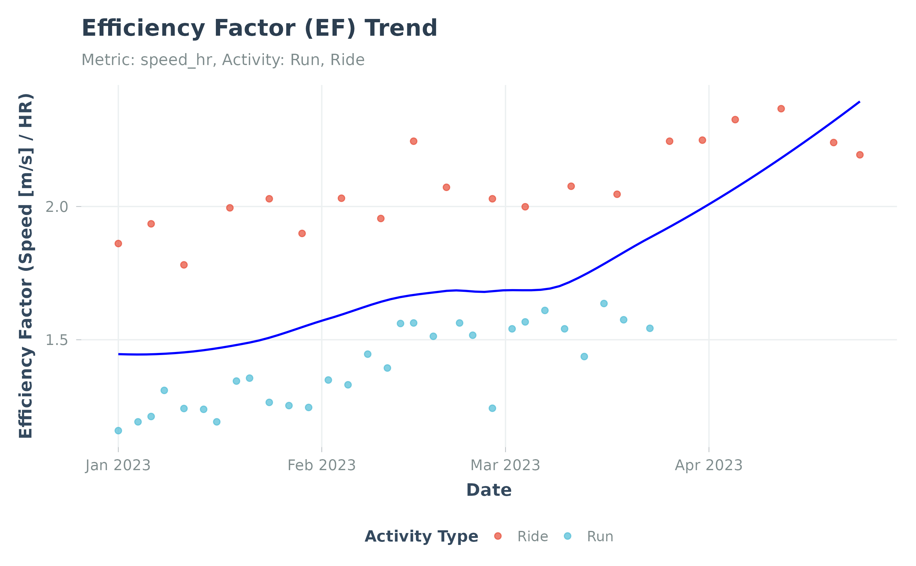

Efficiency Factor trend using sample data

Demo: Separate trend lines per discipline:

# Smooth per activity type to compare trends across disciplines
plot_ef(sample_ef, add_trend_line = TRUE, smooth_per_activity_type = TRUE)
#> `geom_smooth()` using formula = 'y ~ x'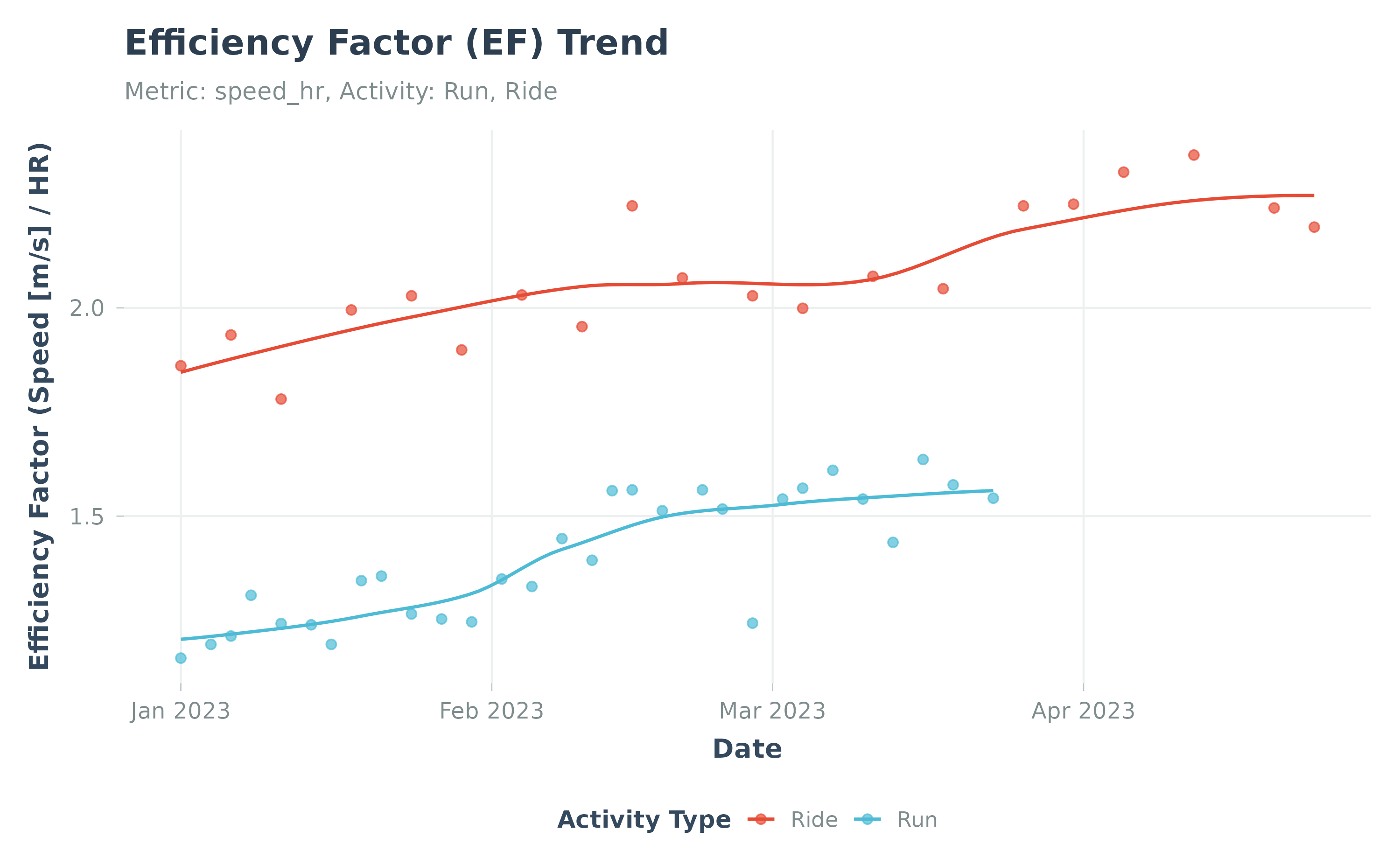

EF with per-discipline smoothing

Interpreting EF

Best Practices:

Track trends over weeks/months, not day-to-day fluctuations
Use steady-state efforts only — Interval workouts will skew results. The package uses coefficient of variation (CV) thresholds to identify steady-state segments, a common approach in exercise physiology (Coyle & González-Alonso, 2001).
Consider external factors — Heat, altitude, fatigue affect EF

Scientific Background: Steady-state exercise is characterized by relatively constant oxygen consumption and heart rate (CV < 8-10%). This package automatically filters non-steady activities to ensure EF calculations reflect true aerobic efficiency rather than pacing artifacts.

See: Coyle, E. F., & González-Alonso, J. (2001). Cardiovascular drift during prolonged exercise. Exercise and Sport Sciences Reviews, 29(2), 88-92. DOI: 10.1097/00003677-200104000-00009; Allen, H., Coggan, A. R., & McGregor, S. (2019). Training and Racing with a Power Meter (3rd ed.). VeloPress. ISBN: 978-1-937715-93-9

Technical Detail: Steady-State Detection Algorithm

Rolling window: A centered rolling window of min(300, N/4) data points (minimum 60 points, ~1-5 minutes at 1 Hz sampling) is applied to the activity stream.
Coefficient of Variation (CV): For each window position, CV = rolling SD / rolling mean is calculated for the primary metric (velocity for running, power for cycling).
Filtering: Data points where CV < steady_cv_threshold (default 8%) are classified as steady-state segments.
Minimum duration: For EF, at least 100 steady-state data points are required. For decoupling, the steady-state segment must span at least min_steady_minutes (default 40 minutes).
Aggregation: EF and decoupling are computed from steady-state data only, using median-based aggregation to reduce sensitivity to outliers.

Practical Analysis:

# Calculate monthly average EF
library(lubridate)

ef_monthly <- ef_runs |>
  mutate(month = floor_date(date, "month")) |>
  group_by(month) |>
  summarise(
    mean_ef = mean(ef_value, na.rm = TRUE),
    n_activities = n()
  ) |>
  arrange(desc(month))

print(ef_monthly)

# Compare first vs last 3 months
recent_ef <- ef_runs |>
  filter(date >= Sys.Date() - 90) |>
  pull(ef_value)
baseline_ef <- ef_runs |>
  filter(date < Sys.Date() - 90, date >= Sys.Date() - 180) |>
  pull(ef_value)

cat(sprintf(
  "Recent EF: %.2f\nBaseline EF: %.2f\nChange: %.1f%%\n",
  mean(recent_ef, na.rm = TRUE),
  mean(baseline_ef, na.rm = TRUE),
  (mean(recent_ef, na.rm = TRUE) / mean(baseline_ef, na.rm = TRUE) - 1) * 100
))

3. Cardiovascular Decoupling

While EF tracks aerobic efficiency across activities over time, decoupling looks within a single activity to measure how efficiency changes from start to finish.

What is Decoupling?

Decoupling quantifies cardiovascular drift—the phenomenon where heart rate gradually rises during prolonged efforts even if pace/power remains constant. Low decoupling indicates good aerobic endurance.

How It Works:

The function compares efficiency (speed/HR or power/HR) between the first half and second half of an activity:

$\text{Decoupling \%} = \frac{\text{EF}_{\text{first half}} - \text{EF}_{\text{second half}}}{\text{EF}_{\text{first half}}} \times 100$

Positive values = efficiency decline in second half (HR drift); <5% commonly used as reference threshold, requires interpretation in context of steady-state and environmental conditions (Coyle & González-Alonso, 2001; Friel, 2009).

Interpretation:

< 5% — Excellent aerobic base, well-adapted
5-10% — Acceptable, some drift but manageable
> 10% — Significant drift (fatigue, heat, insufficient base fitness)

Calculate Decoupling

# For running
decoupling_runs <- calculate_decoupling(
  activities_data = runs,
  activity_type = "Run",
  decouple_metric = "speed_hr",
  min_duration_mins = 60 # Only analyze runs ≥ 60 minutes
)

# For cycling
decoupling_rides <- calculate_decoupling(
  activities_data = rides,
  activity_type = "Ride",
  decouple_metric = "power_hr",
  min_duration_mins = 90 # Longer threshold for cycling
)

# View results
head(decoupling_runs)

Output Columns:

date — Activity date
decoupling — Decoupling percentage (%). Positive = HR drift
status — Calculation status (ok, non_steady, insufficient_data)

Visualizing Decoupling

# Basic plot
plot_decoupling(data = decoupling_runs)

# With trend line
plot_decoupling(data = decoupling_runs, add_trend_line = TRUE)

Demo with Sample Data:

# Load built-in sample data
data("sample_decoupling", package = "Athlytics")

# Plot decoupling trend
plot_decoupling(data = sample_decoupling)
#> `geom_smooth()` using formula = 'y ~ x'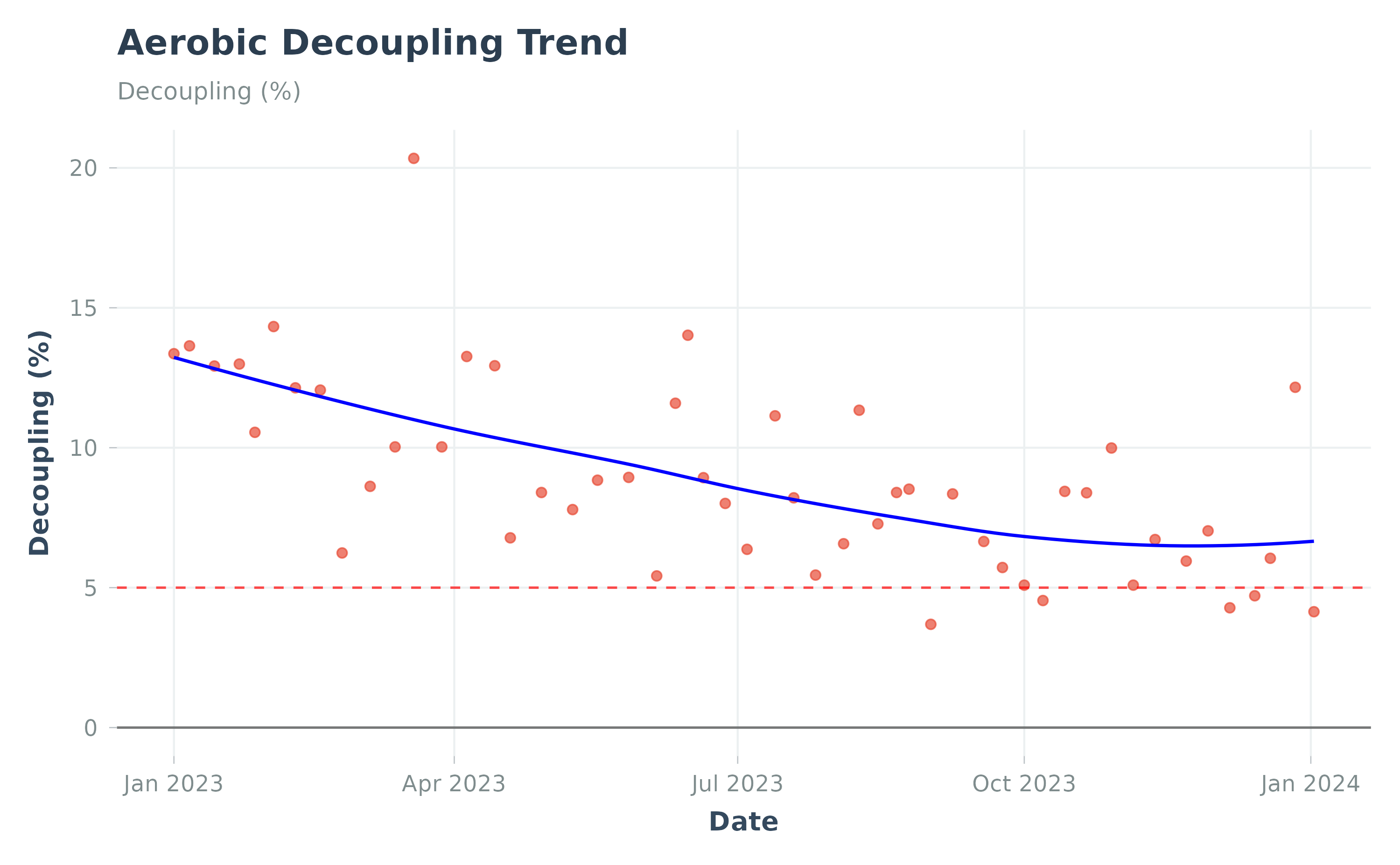

Cardiovascular decoupling using sample data

Practical Applications

1. Assess Aerobic Base:

# Recent decoupling average
recent_decouple <- decoupling_runs |>
  filter(date >= Sys.Date() - 60) |>
  summarise(avg_decouple = mean(decoupling, na.rm = TRUE))

if (recent_decouple$avg_decouple < 5) {
  cat("Excellent aerobic base! Ready for higher intensity.\n")
} else if (recent_decouple$avg_decouple < 10) {
  cat("Good base, continue building aerobic foundation.\n")
} else {
  cat("High decoupling—focus on more easy, long runs.\n")
}

2. Monitor Training Block Progress:

# Compare decoupling over time
library(ggplot2)

decoupling_runs |>
  ggplot(aes(x = date, y = decoupling)) +
  geom_point(alpha = 0.6) +
  geom_smooth(method = "loess", se = TRUE) +
  geom_hline(yintercept = 5, linetype = "dashed", color = "green") +
  geom_hline(yintercept = 10, linetype = "dashed", color = "orange") +
  labs(
    title = "Decoupling Trend Over Time",
    subtitle = "Lower values = better aerobic endurance",
    x = "Date", y = "Decoupling (%)"
  ) +
  theme_minimal()

Important Note: Decoupling is highly affected by environmental conditions (heat, humidity) and cumulative fatigue. Always interpret in context. See: Friel, J. (2009). The Cyclist’s Training Bible (4th ed.). VeloPress — for practical application of decoupling in endurance training.

4. Personal Bests (PBs)

Track your best performances at standard distances over time. Systematic personal best tracking across multiple distances is a well-established method for monitoring endurance performance progression. Analyzing PBs at different distances helps distinguish between improvements in speed (shorter distances) and aerobic endurance (longer distances), aligning with periodization principles (Matveyev, 1981).

Calculate PBs

# Extract personal bests
pbs <- calculate_pbs(
  activities_data = runs,
  activity_type = "Run"
)

# View all PRs
print(pbs)

Supported Distances:

400m, 800m, 1km, 1 mile
5km, 10km
Half marathon, Marathon

Visualize PB Progression

# Plot PR progression
plot_pbs(pbs)

# Filter to specific distance
pbs_5k <- pbs |> filter(distance == "5k")
print(pbs_5k)

Demo with Sample Data:

# Load built-in sample data
data("sample_pbs", package = "Athlytics")

# Plot PB progression
plot_pbs(data = sample_pbs)
#> `geom_smooth()` using formula = 'y ~ x'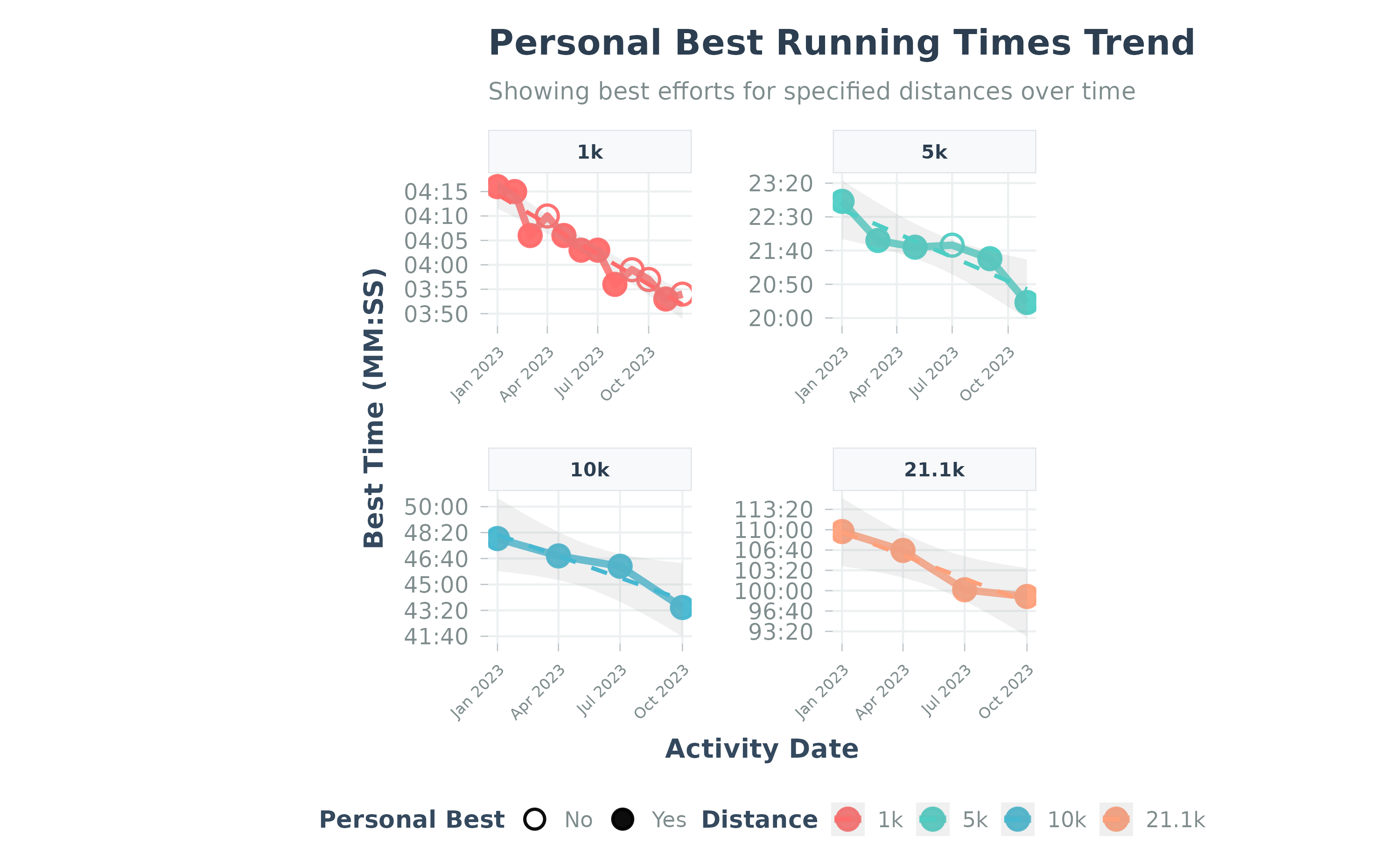

Personal bests progression using sample data

5. Load Exposure Analysis

Visualize your training state in 2D space: acute load vs chronic load.

How does this differ from ACWR? Both use the same underlying data (ATL and CTL), but provide different perspectives:

ACWR collapses acute and chronic load into a single ratio plotted over time — it tells you when load spikes occurred.

Load Exposure preserves the two-dimensional relationship (ATL vs CTL scatter plot) — it tells you where you are in the fitness-fatigue state space, revealing whether a high ACWR comes from ramping up on a low base (risky) or from a natural fluctuation on a high base (less risky).

In practice, use ACWR for day-to-day monitoring and Load Exposure for strategic planning across training phases. Using both together gives a more complete picture than either alone.

Calculate and Plot Exposure

# Calculate exposure
exposure <- calculate_exposure(
  activities_data = runs,
  activity_type = "Run",
  load_metric = "duration_mins"
)

# Plot with risk zones
plot_exposure(data = exposure, risk_zones = TRUE)

Demo with Sample Data:

# Load built-in sample data
data("sample_exposure", package = "Athlytics")

# Plot exposure
plot_exposure(data = sample_exposure)
#> Warning: Removed 27 rows containing missing values or values outside the scale range
#> (`geom_point()`).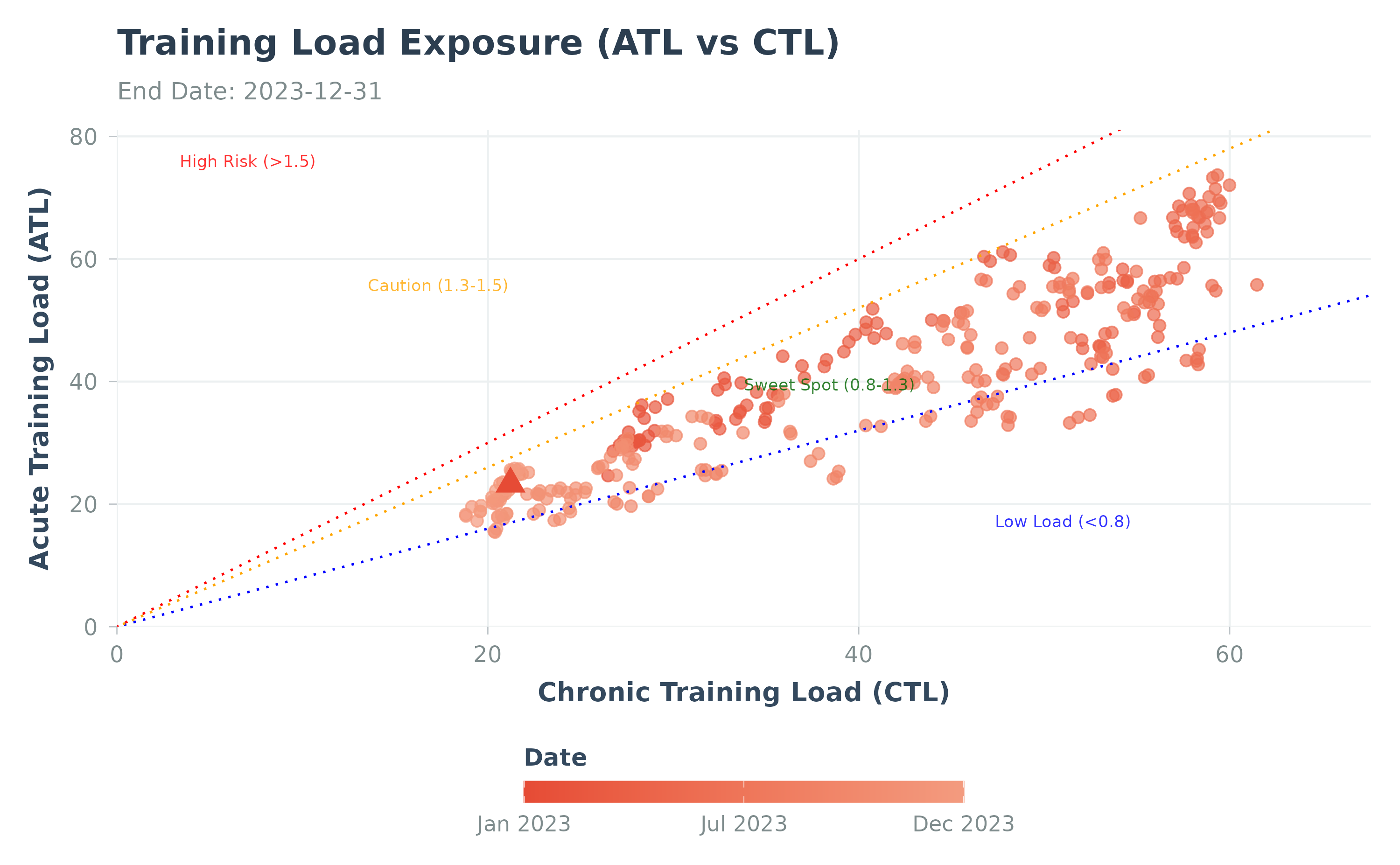

Load exposure analysis using sample data

Interpretation:

Points above diagonal = Acute > chronic (ramping up training)
Points on diagonal = Balanced state
Points below diagonal = Tapering or recovery
Red zone = High ACWR, injury risk

Complete Workflow Example

Here’s a realistic, end-to-end analysis workflow:

library(Athlytics)
library(dplyr)
library(ggplot2)

# ---- 1. Load and Filter Data ----
activities <- load_local_activities("my_strava_export.zip")

# Focus on running activities with HR data
runs <- activities |>
  filter(type == "Run", !is.na(average_heartrate))

cat(sprintf("Loaded %d running activities with HR data\n", nrow(runs)))

# ---- 2. Training Load Monitoring ----
acwr_data <- calculate_acwr(
  activities_data = runs,
  load_metric = "duration_mins"
)

# Check current training status
current_acwr <- acwr_data |>
  filter(date >= Sys.Date() - 30) |>
  tail(1) |>
  pull(acwr_smooth)

cat(sprintf("Current ACWR: %.2f\n", current_acwr))

# Visualize
p1 <- plot_acwr(acwr_data, highlight_zones = TRUE) +
  labs(title = "6-Month Training Load Progression")
print(p1)

# ---- 3. Aerobic Fitness Tracking ----
ef_data <- calculate_ef(
  activities_data = runs,
  ef_metric = "speed_hr"
)

# Calculate fitness trend
ef_trend <- ef_data |>
  mutate(month = lubridate::floor_date(date, "month")) |>
  group_by(month) |>
  summarise(mean_ef = mean(ef_value, na.rm = TRUE))

p2 <- plot_ef(ef_data, add_trend_line = TRUE) +
  labs(title = "Aerobic Efficiency Trend")
print(p2)

# ---- 4. Endurance Assessment ----
# Only for long runs (> 60 min)
decoupling_data <- calculate_decoupling(
  activities_data = runs,
  min_duration_mins = 60
)

avg_decouple <- mean(decoupling_data$decoupling, na.rm = TRUE)
cat(sprintf(
  "Average decoupling: %.1f%% (%s aerobic base)\n",
  avg_decouple,
  ifelse(avg_decouple < 5, "excellent",
    ifelse(avg_decouple < 10, "good", "needs work")
  )
))

p3 <- plot_decoupling(data = decoupling_data) +
  labs(title = "Cardiovascular Drift in Long Runs")
print(p3)

# ---- 5. Export Results ----
# Save plots
ggsave("acwr_analysis.png", plot = p1, width = 10, height = 6, dpi = 300)
ggsave("ef_trend.png", plot = p2, width = 10, height = 6, dpi = 300)
ggsave("decoupling.png", plot = p3, width = 10, height = 6, dpi = 300)

# Export data for further analysis
write.csv(acwr_data, "acwr_results.csv", row.names = FALSE)
write.csv(ef_data, "ef_results.csv", row.names = FALSE)
write.csv(decoupling_data, "decoupling_results.csv", row.names = FALSE)

cat("\nAnalysis complete! Results saved.\n")

Troubleshooting

Common Issues

“No data returned” or empty results

Causes: - Activity type filter doesn’t match your data - Required metrics (e.g., HR) are missing - Date range has no activities

Solutions:

# Check activity types in your data
table(activities$type)

# Check for HR data availability
sum(!is.na(activities$average_heartrate))

# Verify date range
range(activities$date, na.rm = TRUE)

# Try without filtering first
test <- calculate_acwr(activities_data = activities, activity_type = NULL)

“Not enough data for chronic period”

ACWR requires at least 28 days of data. Check your date range:

# How much data do you have?
date_span <- as.numeric(max(activities$date) - min(activities$date))
cat(sprintf("Your data spans %d days\n", date_span))

# If < 28 days, you need more data or use shorter periods

“NA values in output”

Some activities may lack required metrics (HR, power, etc.):

# Filter before calculating
runs_with_hr <- runs |> filter(!is.na(average_heartrate))
ef_data <- calculate_ef(runs_with_hr, ef_metric = "speed_hr")

Plots look strange or empty

# Check if data exists
nrow(acwr_data)
summary(acwr_data$acwr_smooth)

# Try basic R plot first
plot(acwr_data$date, acwr_data$acwr_smooth, type = "l")

Getting Help

Function documentation: ?calculate_acwr, ?plot_ef, etc.
GitHub Issues: Report bugs
Package vignettes: browseVignettes("Athlytics")

Next Steps

Congratulations! You now know how to use all core features of Athlytics.

Advanced Features

Ready to go deeper? Check out:

Advanced Features Tutorial — EWMA-based ACWR with confidence intervals, quality control, and cohort analysis
Function Reference — Complete documentation of all functions

For Researchers

If you’re using Athlytics for research:

Cohort Studies: See calculate_cohort_reference() for multi-athlete percentile comparisons
Data Quality: Use flag_quality() for stream data quality control
Statistical Analysis: All functions return tidy data frames ready for lme4, survival analysis, etc.

Citation

If you use Athlytics in your research, please cite:

@software{athlytics2025,
  title   = {Athlytics: A Computational Framework for Longitudinal Analysis of Exercise Physiology},
  author  = {Zhiang He},
  year    = {2025},
  version = {1.0.4},
  url     = {https://github.com/HzaCode/Athlytics}
}

Session Info

sessionInfo()
#> R version 4.5.2 (2025-10-31)
#> Platform: x86_64-pc-linux-gnu
#> Running under: Ubuntu 24.04.3 LTS
#> 
#> Matrix products: default
#> BLAS:   /usr/lib/x86_64-linux-gnu/openblas-pthread/libblas.so.3 
#> LAPACK: /usr/lib/x86_64-linux-gnu/openblas-pthread/libopenblasp-r0.3.26.so;  LAPACK version 3.12.0
#> 
#> locale:
#>  [1] LC_CTYPE=C.UTF-8       LC_NUMERIC=C           LC_TIME=C.UTF-8       
#>  [4] LC_COLLATE=C.UTF-8     LC_MONETARY=C.UTF-8    LC_MESSAGES=C.UTF-8   
#>  [7] LC_PAPER=C.UTF-8       LC_NAME=C              LC_ADDRESS=C          
#> [10] LC_TELEPHONE=C         LC_MEASUREMENT=C.UTF-8 LC_IDENTIFICATION=C   
#> 
#> time zone: UTC
#> tzcode source: system (glibc)
#> 
#> attached base packages:
#> [1] stats     graphics  grDevices utils     datasets  methods   base     
#> 
#> other attached packages:
#> [1] ggplot2_4.0.2   Athlytics_1.0.4
#> 
#> loaded via a namespace (and not attached):
#>  [1] Matrix_1.7-4       gtable_0.3.6       jsonlite_2.0.0     dplyr_1.2.0       
#>  [5] compiler_4.5.2     tidyselect_1.2.1   jquerylib_0.1.4    splines_4.5.2     
#>  [9] systemfonts_1.3.1  scales_1.4.0       textshaping_1.0.4  yaml_2.3.12       
#> [13] fastmap_1.2.0      lattice_0.22-7     R6_2.6.1           labeling_0.4.3    
#> [17] generics_0.1.4     knitr_1.51         htmlwidgets_1.6.4  tibble_3.3.1      
#> [21] desc_1.4.3         lubridate_1.9.5    bslib_0.10.0       pillar_1.11.1     
#> [25] RColorBrewer_1.1-3 rlang_1.1.7        cachem_1.1.0       xfun_0.56         
#> [29] fs_1.6.6           sass_0.4.10        S7_0.2.1           otel_0.2.0        
#> [33] timechange_0.4.0   cli_3.6.5          mgcv_1.9-3         withr_3.0.2       
#> [37] pkgdown_2.2.0      magrittr_2.0.4     digest_0.6.39      grid_4.5.2        
#> [41] nlme_3.1-168       lifecycle_1.0.5    vctrs_0.7.1        evaluate_1.0.5    
#> [45] glue_1.8.0         farver_2.1.2       ragg_1.5.0         rmarkdown_2.30    
#> [49] tools_4.5.2        pkgconfig_2.0.3    htmltools_0.5.9

Athlytics Package

2026-02-20

Welcome to Athlytics

Prerequisites

Installation

Your Strava Data Export

Loading Your Data

Basic Loading

Understanding the Data Structure

Data Quality Checks

Filtering Your Data

Core Analyses

1. Training Load (ACWR)

Basic ACWR Calculation

Visualizing ACWR

Risk Zones

Interpreting Your ACWR

Choosing Load Metrics

Important Caveats

2. Efficiency Factor (EF)

Calculate EF

Visualizing EF Trends

Interpreting EF

3. Cardiovascular Decoupling

Calculate Decoupling

Visualizing Decoupling

Practical Applications

4. Personal Bests (PBs)

Calculate PBs

Visualize PB Progression

5. Load Exposure Analysis

Calculate and Plot Exposure

Complete Workflow Example

Troubleshooting

Common Issues

“No data returned” or empty results

“Not enough data for chronic period”

“NA values in output”

Plots look strange or empty

Getting Help

Next Steps

Advanced Features

For Researchers

Citation

Session Info