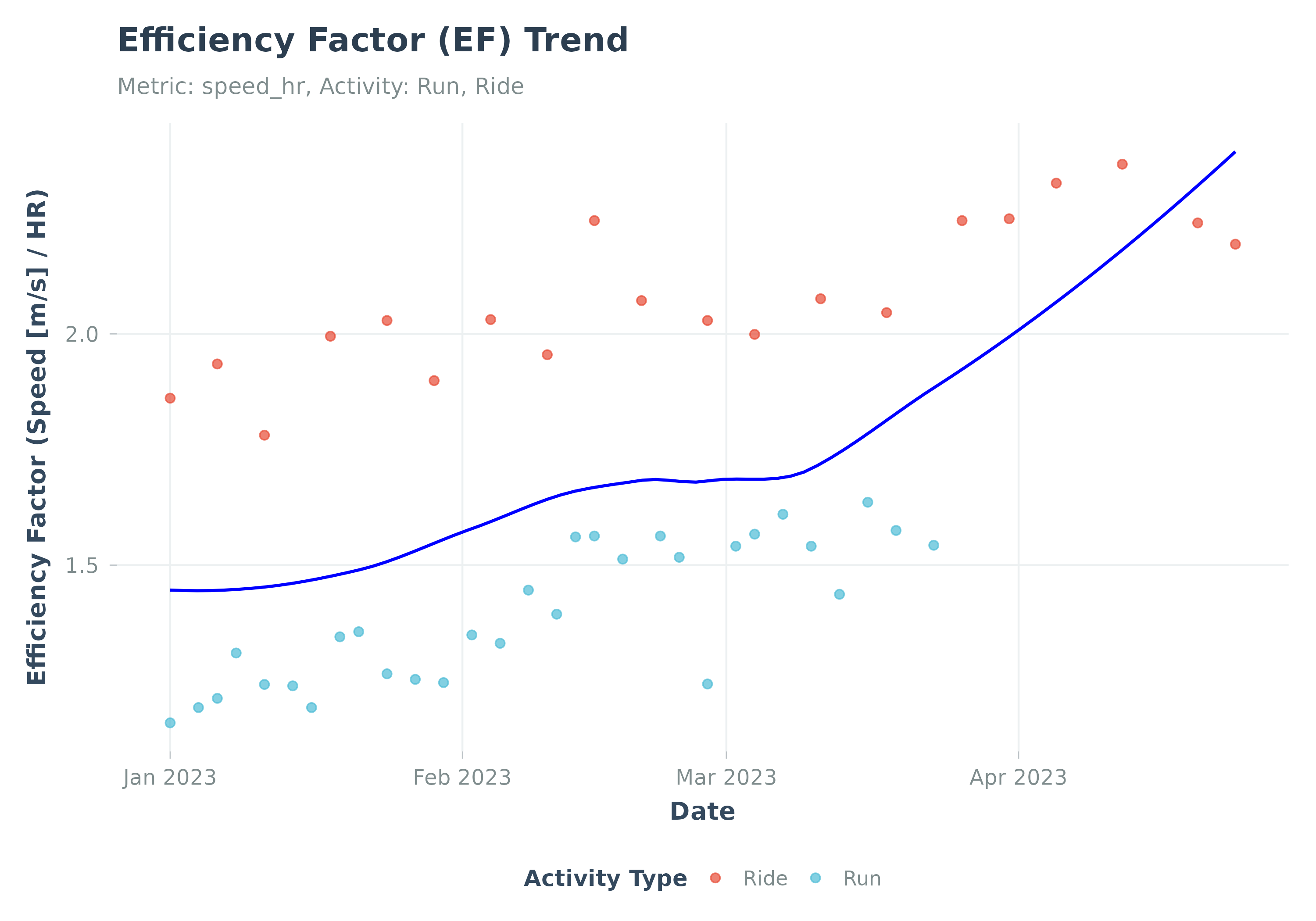
Plot Efficiency Factor (EF) Trend — plot

Visualizes the trend of Efficiency Factor (EF) over time.

Usage

plot_ef(
  data,
  add_trend_line = TRUE,
  smoothing_method = "loess",
  smooth_per_activity_type = FALSE,
  group_var = NULL,
  group_colors = NULL,
  title = NULL,
  subtitle = NULL,
  ...
)

Arguments

data: A data frame from calculate_ef(). Must contain date, ef_value, and activity_type columns.
add_trend_line: Add a smoothed trend line (geom_smooth)? Default TRUE.
smoothing_method: Smoothing method for trend line (e.g., "loess", "lm"). Default "loess".
smooth_per_activity_type: Logical. If TRUE and add_trend_line = TRUE, draws separate trend lines for each activity type. Default FALSE (single trend line for all data). Note: this parameter only applies when group_var = NULL. When group_var is set, smoothing is always done per group and this parameter is ignored with a warning.
group_var: Optional. Column name for grouping/faceting (e.g., "athlete_id").
group_colors: Optional. Named vector of colors for groups.
title: Optional. Custom title for the plot.
subtitle: Optional. Custom subtitle for the plot.
...: Additional arguments. Arguments activity_type, ef_metric, start_date, end_date, min_duration_mins, ef_df are deprecated and ignored.

Value

A ggplot object showing the EF trend.

Details

Plots EF (output/HR based on activity averages). Best practice: Use calculate_ef() first, then pass the result to this function.

Examples

# Example using pre-calculated sample data
data("sample_ef", package = "Athlytics")
p <- plot_ef(sample_ef)
print(p)
#> `geom_smooth()` using formula = 'y ~ x'