Examples
Here you’ll find a series of example of calls to yf_get(). Most arguments are self-explanatory, but you can find more details at the help files.
The steps of the algorithm are:
- check cache files for existing data
- if not in cache, fetch stock prices from YF and clean up the raw data
- write cache file if not available
- calculate all returns
- build diagnostics
- return the data to the user
Fetching a single stock price
library(yfR)

# set options for algorithm
my_ticker <- 'FB'
first_date <- Sys.Date() - 30
last_date <- Sys.Date()

# fetch data
df_yf <- yf_get(tickers = my_ticker,
                first_date = first_date,
                last_date = last_date)

# output is a tibble with data
head(df_yf)
## # A tibble: 6 × 11
## ticker ref_date price_open price_high price_low price_close volume
## <chr> <date> <dbl> <dbl> <dbl> <dbl> <dbl>
## 1 FB 2022-05-16 197. 205. 196. 200. 27112595
## 2 FB 2022-05-17 202. 205. 198. 203. 24872729
## 3 FB 2022-05-18 200 201 192. 192. 23959966
## 4 FB 2022-05-19 191. 195. 190. 191. 24446938
## 5 FB 2022-05-20 195. 198. 188. 194. 31465570
## 6 FB 2022-05-23 195. 197. 191. 196. 25059161
## # … with 4 more variables: price_adjusted <dbl>, ret_adjusted_prices <dbl>,
## # ret_closing_prices <dbl>, cumret_adjusted_prices <dbl>Fetching many stock prices
library(yfR)
library(ggplot2)

my_ticker <- c('FB', 'GM', 'MMM')
first_date <- Sys.Date() - 100
last_date <- Sys.Date()

df_yf_multiple <- yf_get(tickers = my_ticker,
                         first_date = first_date,
                         last_date = last_date)


p <- ggplot(df_yf_multiple, aes(x = ref_date, y = price_adjusted,
                                color = ticker)) +
  geom_line()

p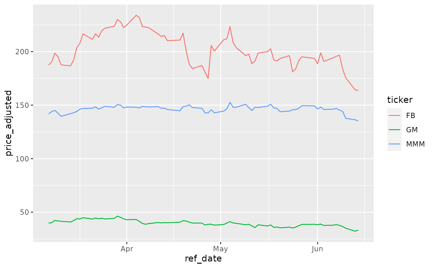
Fetching daily/weekly/monthly/yearly price data
library(yfR)
library(ggplot2)
library(dplyr)

my_ticker <- 'GE'
first_date <- '2005-01-01'
last_date <- Sys.Date()

df_dailly <- yf_get(tickers = my_ticker,
                    first_date, last_date,
                    freq_data = 'daily') %>%
  mutate(freq = 'daily')

df_weekly <- yf_get(tickers = my_ticker,
                    first_date, last_date,
                    freq_data = 'weekly') %>%
  mutate(freq = 'weekly')

df_monthly <- yf_get(tickers = my_ticker,
                     first_date, last_date,
                     freq_data = 'monthly') %>%
  mutate(freq = 'monthly')

df_yearly <- yf_get(tickers = my_ticker,
                    first_date, last_date,
                    freq_data = 'yearly') %>%
  mutate(freq = 'yearly')

# bind it all together for plotting
df_allfreq <- bind_rows(
  list(df_dailly, df_weekly, df_monthly, df_yearly)
) %>%
  mutate(freq = factor(freq,
                       levels = c('daily',
                                  'weekly',
                                  'monthly',
                                  'yearly'))) # make sure the order in plot is right

p <- ggplot(df_allfreq, aes(x = ref_date, y = price_adjusted)) +
  geom_line() +
  facet_grid(freq ~ ticker) +
  theme_minimal() +
  labs(x = '', y = 'Adjusted Prices')

print(p)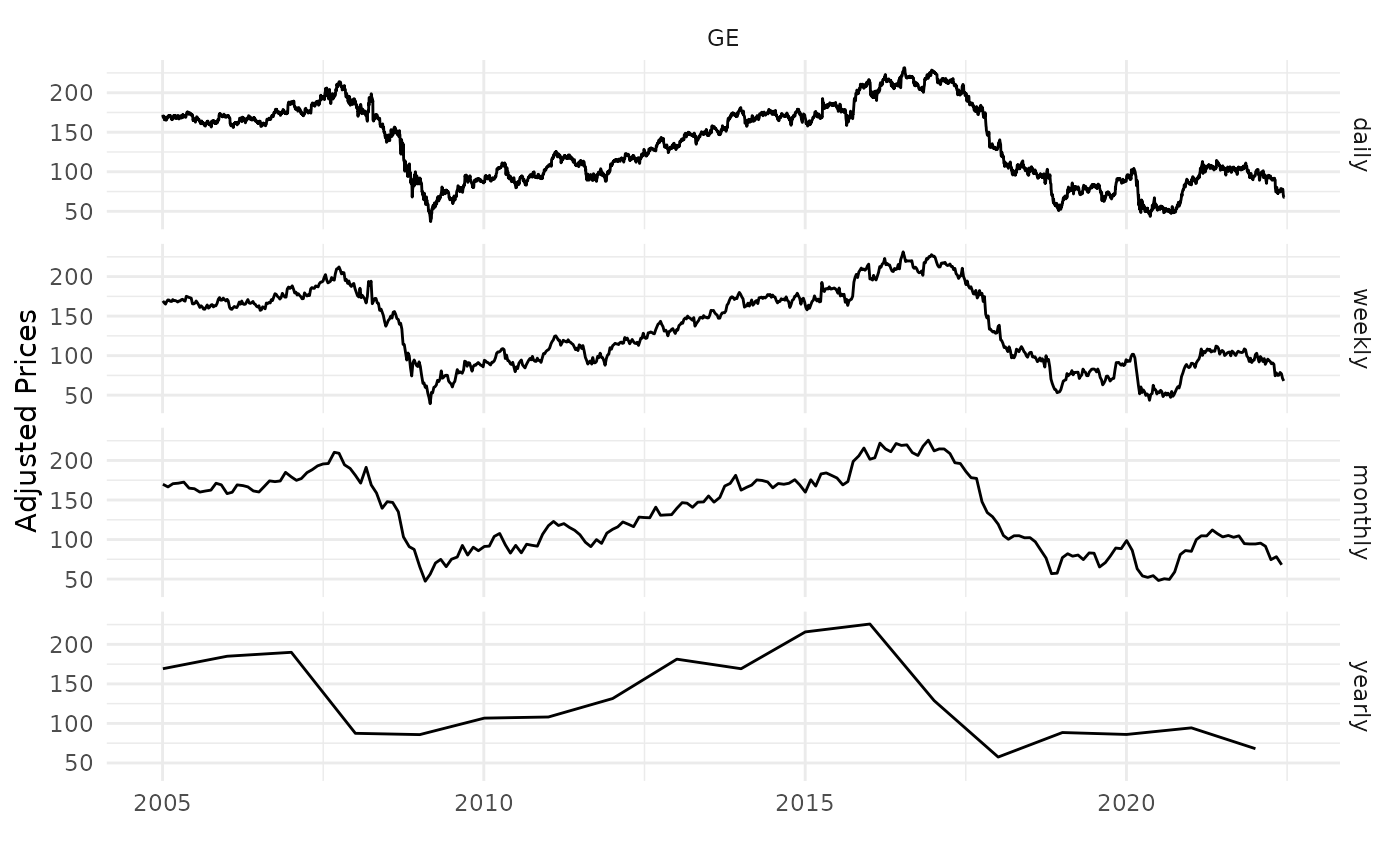
Changing format to wide
library(yfR)
library(ggplot2)

my_ticker <- c('FB', 'GM', 'MMM')
first_date <- Sys.Date() - 100
last_date <- Sys.Date()

df_yf_multiple <- yf_get(tickers = my_ticker,
                         first_date = first_date,
                         last_date = last_date)

print(df_yf_multiple)
## # A tibble: 210 × 11
## ticker ref_date price_open price_high price_low price_close volume
## * <chr> <date> <dbl> <dbl> <dbl> <dbl> <dbl>
## 1 FB 2022-03-07 201. 201. 187. 187. 38560609
## 2 FB 2022-03-08 188. 197. 186. 190. 37508149
## 3 FB 2022-03-09 196. 199. 194. 198. 31894695
## 4 FB 2022-03-10 195. 196. 191. 195. 24852975
## 5 FB 2022-03-11 193. 194. 187. 188. 34694534
## 6 FB 2022-03-14 187. 192. 186. 187. 31010462
## 7 FB 2022-03-15 191. 192. 186. 192. 31721682
## 8 FB 2022-03-16 195. 204. 195. 204. 40640264
## 9 FB 2022-03-17 202. 208. 201. 208. 29499681
## 10 FB 2022-03-18 207. 217. 206 216. 52127982
## # … with 200 more rows, and 4 more variables: price_adjusted <dbl>,
## # ret_adjusted_prices <dbl>, ret_closing_prices <dbl>,
## # cumret_adjusted_prices <dbl>
l_wide <- yf_convert_to_wide(df_yf_multiple)

names(l_wide)
## [1] "price_open" "price_high" "price_low"
## [4] "price_close" "volume" "price_adjusted"
## [7] "ret_adjusted_prices" "ret_closing_prices" "cumret_adjusted_prices"
prices_wide <- l_wide$price_adjusted
head(prices_wide)
## # A tibble: 6 × 4
## ref_date FB GM MMM
## <date> <dbl> <dbl> <dbl>
## 1 2022-03-07 187. 39.8 142.
## 2 2022-03-08 190. 40.2 144.
## 3 2022-03-09 198. 42.3 145.
## 4 2022-03-10 195. 41.8 142.
## 5 2022-03-11 188. 41.5 140.
## 6 2022-03-14 187. 40.8 142.