Analyzing B3 Index Data • rb3

Introduction

The B3 (Brasil, Bolsa, Balcão) provides comprehensive data for its market indices through various endpoints. These indices represent essential benchmarks for the Brazilian financial market, measuring the performance of different market segments.

The rb3 package simplifies access to this data through four key templates:

b3-indexes-historical-data: Historical performance data for B3 indices
b3-indexes-composition: Composition of all B3 indices showing which stocks belong to each index
b3-indexes-theoretical-portfolio: Theoretical portfolio weights for indices with detailed component weights
b3-indexes-current-portfolio: Current actual portfolio with additional sector classification information

This vignette demonstrates how to retrieve, analyze, and visualize index data using the rb3 package, featuring examples for the most popular indices like Ibovespa (IBOV), Small Caps (SMLL), and Dividend Index (IDIV).

library(rb3)
library(dplyr)
library(ggplot2)
library(tidyr)
library(stringr)
library(lubridate)

Retrieving available indices

The rb3 package provides a function to retrieve all available indices from B3:

# Get all available indices
indexes <- indexes_get()
head(indexes)

#> [1] "AGFS" "BDRX" "GPTW" "IBBR" "IBEE" "IBEP"

These codes represent the various indices calculated and published by B3. Some of the most important ones include:

IBOV: Ibovespa - the main Brazilian stock market index
SMLL: Small Caps Index - represents smaller market capitalization stocks
IDIV: Dividend Index - tracks stocks with the best dividend payment policy
IBXX: IBrX-100 - represents the 100 most traded stocks
IBXL: IBrX-50 - represents the 50 most traded stocks
IBRA: Brazil Broad-Based Index - broader market index

Fetching historical index data

To analyze the historical performance of indices, you can use the b3-indexes-historical-data template:

# Download historical data for specific indices across multiple years
fetch_marketdata("b3-indexes-historical-data",
  throttle = TRUE,
  index = c("IBOV", "SMLL", "IDIV"),
  year = 2018:2023
)

After downloading, you can retrieve and analyze the data:

# Get the historical data for analysis
index_history <- indexes_historical_data_get() |>
  filter(
    symbol %in% c("IBOV", "SMLL", "IDIV"),
    refdate >= "2018-01-01"
  ) |>
  collect()

Visualizing index performance

Let’s compare the performance of multiple indices over time:

# Calculate the normalized performance (setting the starting point to 100)
index_performance <- index_history |>
  group_by(symbol) |>
  arrange(refdate) |>
  mutate(
    norm_value = value / first(value) * 100
  )

# Create the performance chart
ggplot(index_performance, aes(x = refdate, y = norm_value, color = symbol)) +
  geom_line(linewidth = 1) +
  labs(
    title = "Comparative Performance of B3 Indices",
    subtitle = "Normalized values (starting at 100)",
    x = "Date",
    y = "Normalized Value",
    color = "Index"
  ) +
  theme_light() +
  scale_x_date(date_labels = "%b %Y", date_breaks = "6 months") +
  theme(axis.text.x = element_text(angle = 45, hjust = 1))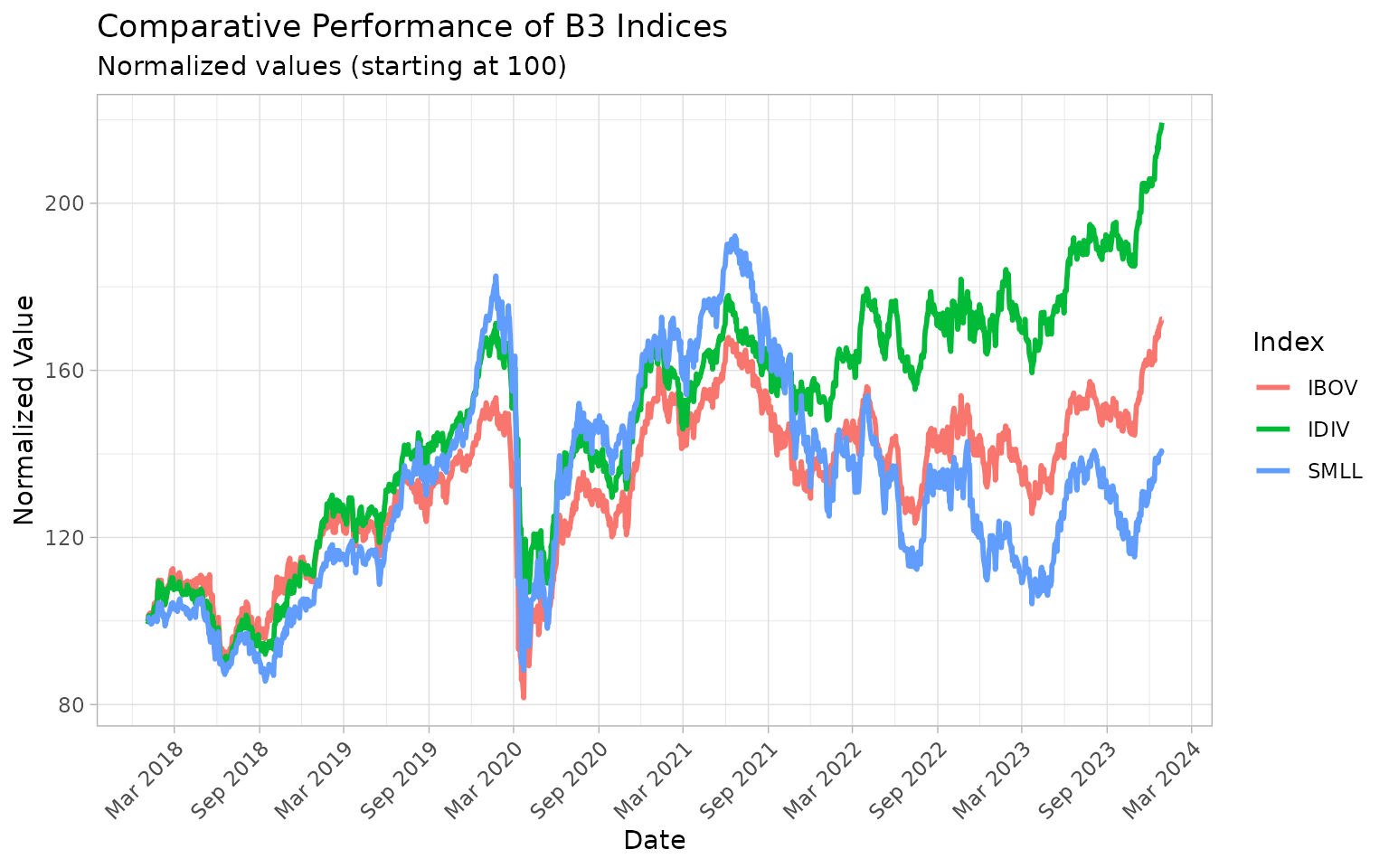

Historical Performance of B3 Indices (2018-2023)

This chart shows the relative performance of the selected indices, allowing you to compare their movements regardless of their absolute values.

Analyzing index composition

The b3-indexes-composition template provides data about which stocks belong to each index:

# Download index composition data
fetch_marketdata("b3-indexes-composition")

After downloading, you can retrieve the composition data:

# Get the composition data
composition <- indexes_composition_get() |>
  collect()

# Display a subset of the composition data
head(composition)
#> # A tibble: 6 × 3
#>   update_date symbol indexes                                     
#>   <date>      <chr>  <chr>                                       
#> 1 2025-04-14  TTEN3  AGFS,IBRA,ICO2,ICON,IGCT,IGCX,IGNM,ITAG,SMLL
#> 2 2025-04-14  ABBV34 BDRX                                        
#> 3 2025-04-14  ABCB4  IBRA,ICO2,IDIV,IFNC,IGCT,IGCX,ITAG,SMLL     
#> 4 2025-04-14  ADBE34 BDRX                                        
#> 5 2025-04-14  A1AP34 BDRX                                        
#> 6 2025-04-14  A1MD34 BDRX

Finding stocks in multiple indices

You can analyze which stocks appear in multiple key indices:

# Get stocks in specific indices
selected_indices <- c("IBOV", "SMLL", "IDIV")

# Find stocks in each index
stocks_by_index <- lapply(selected_indices, function(idx) {
  composition |>
    filter(update_date == latest_date, str_detect(indexes, idx)) |>
    pull(symbol)
})
names(stocks_by_index) <- selected_indices

# Create a data frame for the Venn diagram visualization
index_overlaps <- data.frame(
  Index = c(
    "IBOV only", "SMLL only", "IDIV only",
    "IBOV & SMLL", "IBOV & IDIV", "SMLL & IDIV",
    "All three indices"
  ),
  Count = c(
    length(setdiff(setdiff(stocks_by_index$IBOV, stocks_by_index$SMLL), stocks_by_index$IDIV)),
    length(setdiff(setdiff(stocks_by_index$SMLL, stocks_by_index$IBOV), stocks_by_index$IDIV)),
    length(setdiff(setdiff(stocks_by_index$IDIV, stocks_by_index$IBOV), stocks_by_index$SMLL)),
    length(intersect(setdiff(stocks_by_index$IBOV, stocks_by_index$IDIV), stocks_by_index$SMLL)),
    length(intersect(setdiff(stocks_by_index$IBOV, stocks_by_index$SMLL), stocks_by_index$IDIV)),
    length(intersect(setdiff(stocks_by_index$SMLL, stocks_by_index$IBOV), stocks_by_index$IDIV)),
    length(Reduce(intersect, stocks_by_index))
  )
)

# Create a bar chart to visualize overlaps
ggplot(index_overlaps, aes(x = reorder(Index, Count), y = Count)) +
  geom_bar(stat = "identity", fill = "steelblue") +
  coord_flip() +
  labs(
    title = "Stock Overlap Between Major B3 Indices",
    subtitle = paste("As of", latest_date),
    x = NULL,
    y = "Number of Stocks"
  ) +
  theme_light() +
  geom_text(aes(label = Count), hjust = -0.2)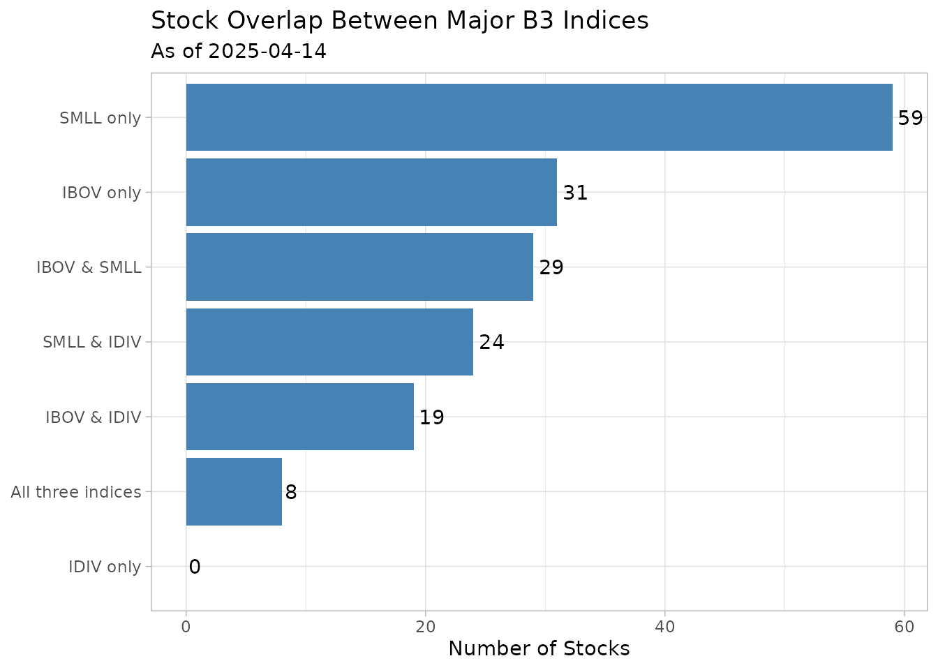

Overlapping Stocks Between Major B3 Indices

Finding which indices contain a specific stock

You can also determine which indices include a specific stock:

# Find all indices that include a specific stock
find_indices_for_stock <- function(stock_symbol, comp_data, date) {
  comp_data |>
    filter(update_date == date, symbol == stock_symbol) |>
    pull(indexes) |>
    str_split(",") |>
    unlist() |>
    sort()
}

# Example: Find indices containing PETR4
petr4_indices <- find_indices_for_stock("PETR4", composition, latest_date)

#>  [1] "IBBR" "IBEE" "IBEW" "IBLV" "IBOV" "IBRA" "IBSD" "IBXL" "IBXX" "IDIV"
#> [11] "IDVR" "IGCT" "IGCX" "ITAG" "MLCX"

Analyzing index weights with the theoretical portfolio

The b3-indexes-theoretical-portfolio template provides information about the weights of stocks in each index:

# Download theoretical portfolio data
fetch_marketdata("b3-indexes-theoretical-portfolio", index = c("IBOV", "SMLL", "IDIV"))

After downloading, you can retrieve and analyze the portfolio weights:

# Get the theoretical portfolio data
theoretical <- indexes_theoretical_portfolio_get() |>
  collect()

# Get the latest date for each index
latest_dates <- theoretical |>
  group_by(index) |>
  summarise(latest = max(refdate))

Top constituents by weight

You can analyze the top constituents of an index by weight:

# Get the top 10 constituents by weight for IBOV
ibov_top10 <- theoretical |>
  filter(index == "IBOV", refdate == latest_dates$latest[latest_dates$index == "IBOV"]) |>
  arrange(desc(weight)) |>
  slice_head(n = 10)

# Create a bar chart of top constituents
ggplot(ibov_top10, aes(x = reorder(symbol, weight), y = weight)) +
  geom_bar(stat = "identity", fill = "darkblue") +
  coord_flip() +
  labs(
    title = "Top 10 Constituents by Weight in Ibovespa",
    subtitle = paste("As of", latest_dates$latest[latest_dates$index == "IBOV"]),
    x = NULL,
    y = "Weight (%)"
  ) +
  theme_light() +
  scale_y_continuous(labels = scales::percent) +
  geom_text(aes(label = scales::percent(weight, accuracy = 0.01)), hjust = -0.2)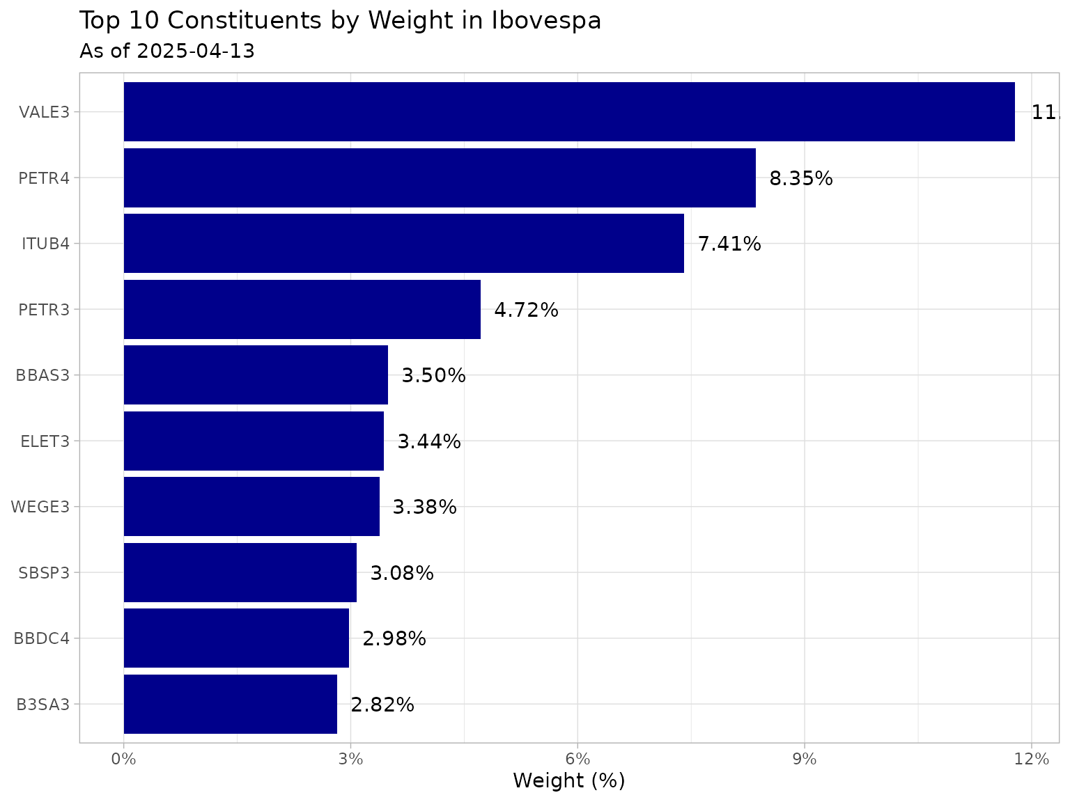

Top 10 Constituents by Weight in Ibovespa

Comparing index concentration

You can compare the concentration of different indices by analyzing their weight distribution:

# Calculate cumulative weights for different indices
concentration_data <- list()

for (idx in c("IBOV", "SMLL", "IDIV")) {
  latest <- latest_dates$latest[latest_dates$index == idx]

  index_weights <- theoretical |>
    filter(index == idx, refdate == latest) |>
    arrange(desc(weight))

  total_stocks <- nrow(index_weights)

  concentration_data[[idx]] <- data.frame(
    index = idx,
    top_n = c(1, 5, 10, 20, total_stocks),
    cum_weight = c(
      sum(index_weights$weight[1:1]),
      sum(index_weights$weight[1:5]),
      sum(index_weights$weight[1:10]),
      sum(index_weights$weight[1:20]),
      sum(index_weights$weight)
    )
  )
}

concentration_df <- bind_rows(concentration_data)

# Create a grouped bar chart
concentration_plot <- concentration_df |>
  filter(top_n %in% c(1, 5, 10, 20)) |>
  mutate(top_n_label = paste("Top", top_n))

ggplot(concentration_plot, aes(x = index, y = cum_weight, fill = factor(top_n))) +
  geom_bar(stat = "identity", position = "dodge") +
  labs(
    title = "Index Concentration Analysis",
    subtitle = "Cumulative weight of top constituents",
    x = NULL,
    y = "Cumulative Weight",
    fill = "Number of Stocks"
  ) +
  theme_light() +
  scale_y_continuous(labels = scales::percent) +
  scale_fill_brewer(palette = "Blues", labels = c("Top 1", "Top 5", "Top 10", "Top 20"))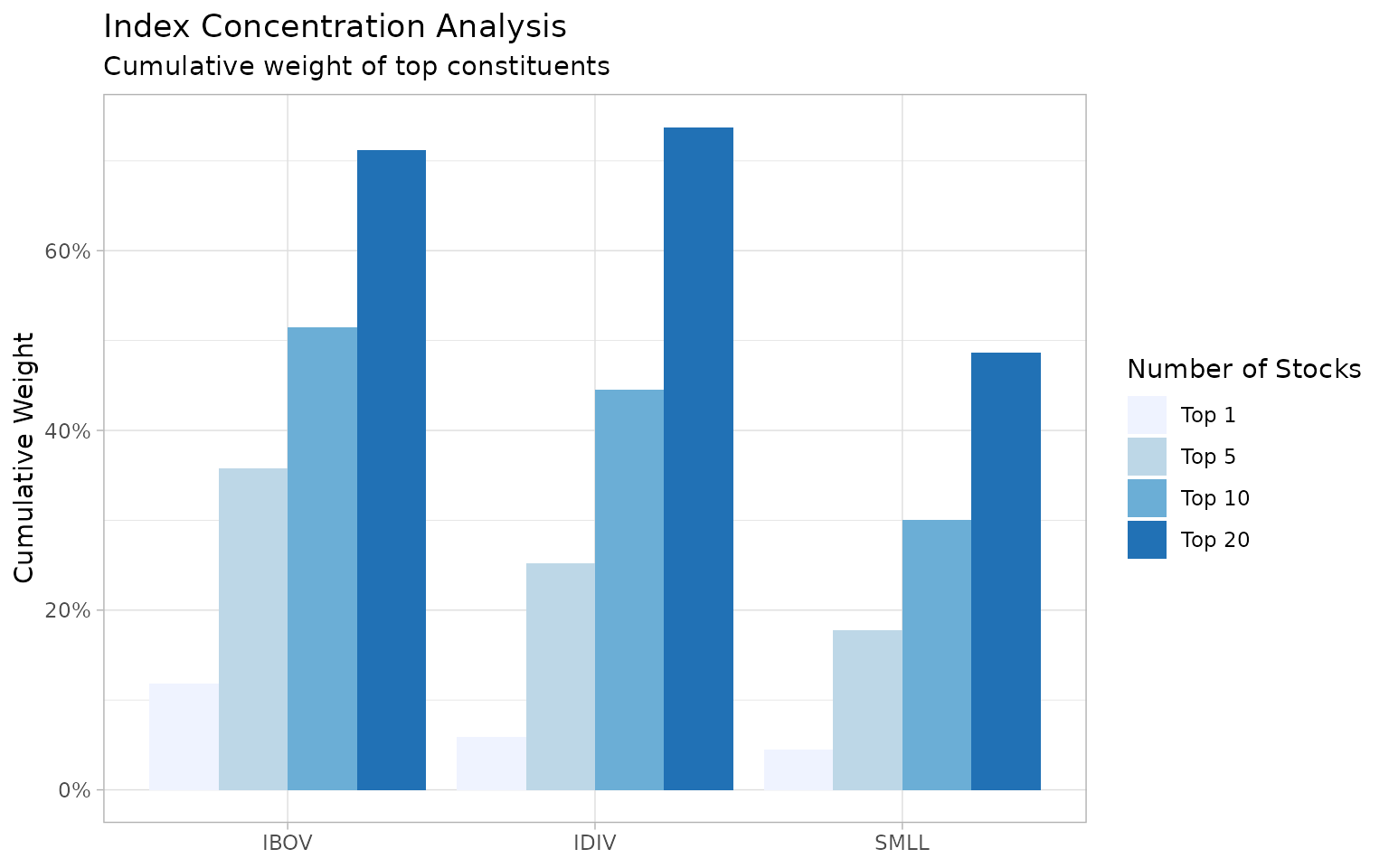

Weight Concentration in B3 Indices

This chart shows how concentrated each index is, revealing differences in their construction methodology.

Sector analysis with the current portfolio

The b3-indexes-current-portfolio template provides the actual current portfolio with additional sector classification:

# Download current portfolio data
fetch_marketdata("b3-indexes-current-portfolio", index = c("IBOV", "SMLL", "IDIV"))

After downloading, you can retrieve the data:

# Get the current portfolio data
current <- indexes_current_portfolio_get() |>
  collect()

# Get the latest date for each index
current_latest <- current |>
  group_by(index) |>
  summarise(latest = max(refdate))

Sector composition analysis

You can analyze the sector composition of different indices:

# Create sector breakdown for each index
sector_data <- list()

for (idx in c("IBOV", "SMLL", "IDIV")) {
  latest <- current_latest$latest[current_latest$index == idx]

  sector_data[[idx]] <- current |>
    filter(index == idx, refdate == latest) |>
    group_by(sector) |>
    summarise(weight = sum(weight)) |>
    arrange(desc(weight)) |>
    mutate(index = idx)
}

sector_df <- bind_rows(sector_data)

# Create a grouped bar chart for sector comparison
ggplot(sector_df, aes(x = index, y = weight, fill = sector)) +
  geom_bar(stat = "identity") +
  labs(
    title = "Sector Composition of B3 Indices",
    subtitle = paste("As of", format(max(current_latest$latest), "%b %Y")),
    x = NULL,
    y = "Weight",
    fill = "Sector"
  ) +
  theme_light() +
  scale_y_continuous(labels = scales::percent) +
  coord_flip() +
  theme(legend.position = "bottom", legend.box = "horizontal")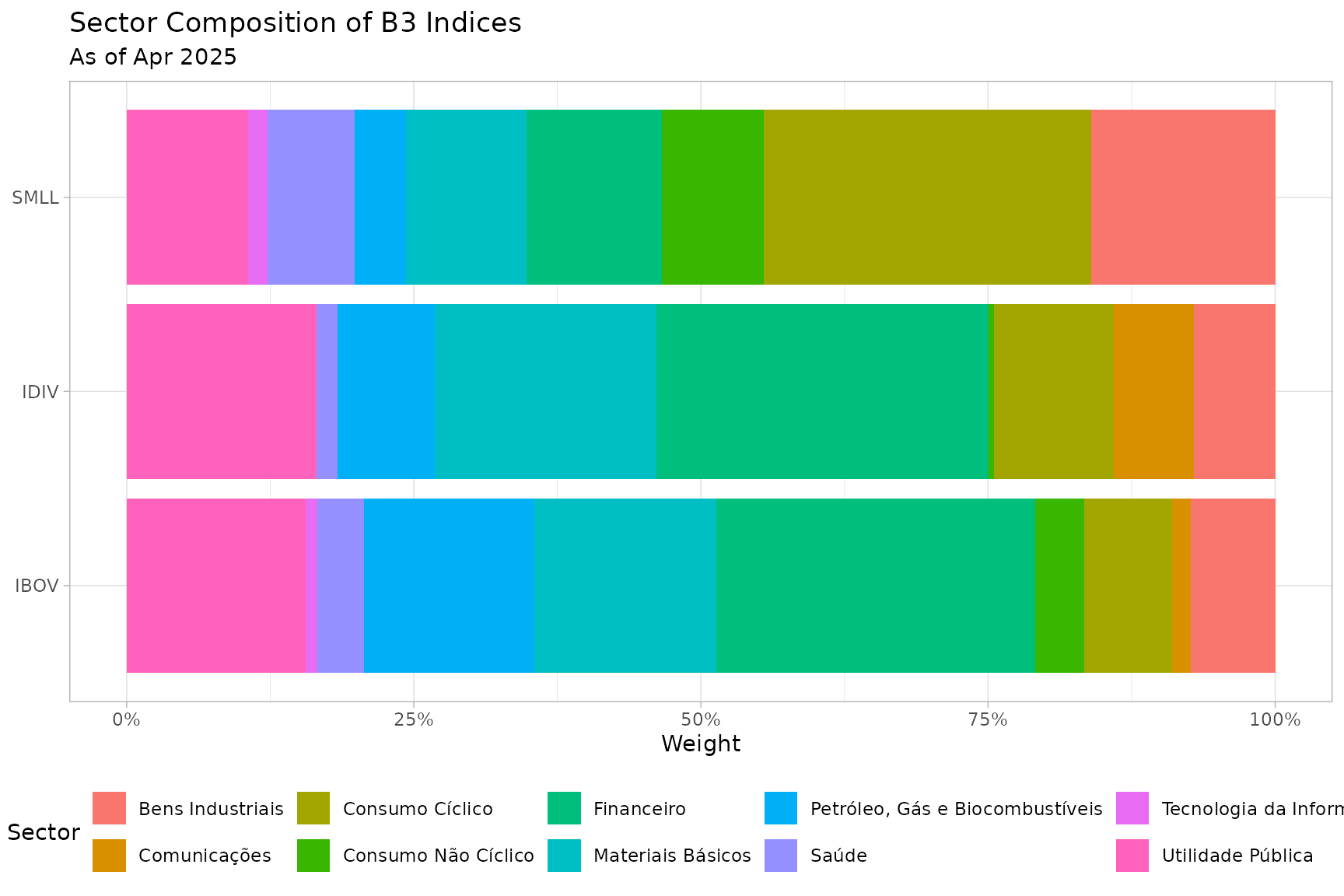

Sector Breakdown of B3 Indices

This visualization shows how sector exposure varies across different indices, which is important for diversification analysis.

Creating helper functions for index analysis

You can create helper functions to streamline common tasks:

# Function to get assets in specific indices
indexes_assets_by_indexes <- function(index_list) {
  last_date <- indexes_composition_get() |>
    summarise(update_date = max(update_date)) |>
    collect() |>
    pull(update_date)

  x <- lapply(index_list, function(idx) {
    indexes_composition_get() |>
      filter(update_date == last_date, str_detect(indexes, idx)) |>
      select(symbol) |>
      collect() |>
      pull(symbol)
  })
  stats::setNames(x, index_list)
}

# Function to find which indices contain specific assets
indexes_indexes_by_assets <- function(symbols) {
  last_date <- indexes_composition_get() |>
    summarise(update_date = max(update_date)) |>
    collect() |>
    pull(update_date)

  indexes_composition_get() |>
    filter(update_date == last_date, symbol %in% symbols) |>
    select(symbol, indexes) |>
    collect() |>
    mutate(
      indexes_list = str_split(indexes, ",")
    )
}

Analyzing index performance metrics

You can calculate various performance metrics for the indices:

# Calculate monthly returns
monthly_returns <- index_history |>
  group_by(symbol) |>
  arrange(refdate) |>
  mutate(
    year_month = floor_date(refdate, "month"),
    monthly_return = value / lag(value) - 1
  ) |>
  filter(!is.na(monthly_return)) |>
  group_by(symbol, year_month) |>
  summarise(
    monthly_return = last(monthly_return),
    .groups = "drop"
  )

# Visualize the monthly returns
ggplot(monthly_returns, aes(x = year_month, y = monthly_return, fill = symbol)) +
  geom_bar(stat = "identity", position = "dodge") +
  facet_wrap(~symbol, ncol = 1) +
  labs(
    title = "Monthly Returns of B3 Indices",
    x = NULL,
    y = "Monthly Return"
  ) +
  theme_light() +
  scale_y_continuous(labels = scales::percent) +
  theme(legend.position = "none")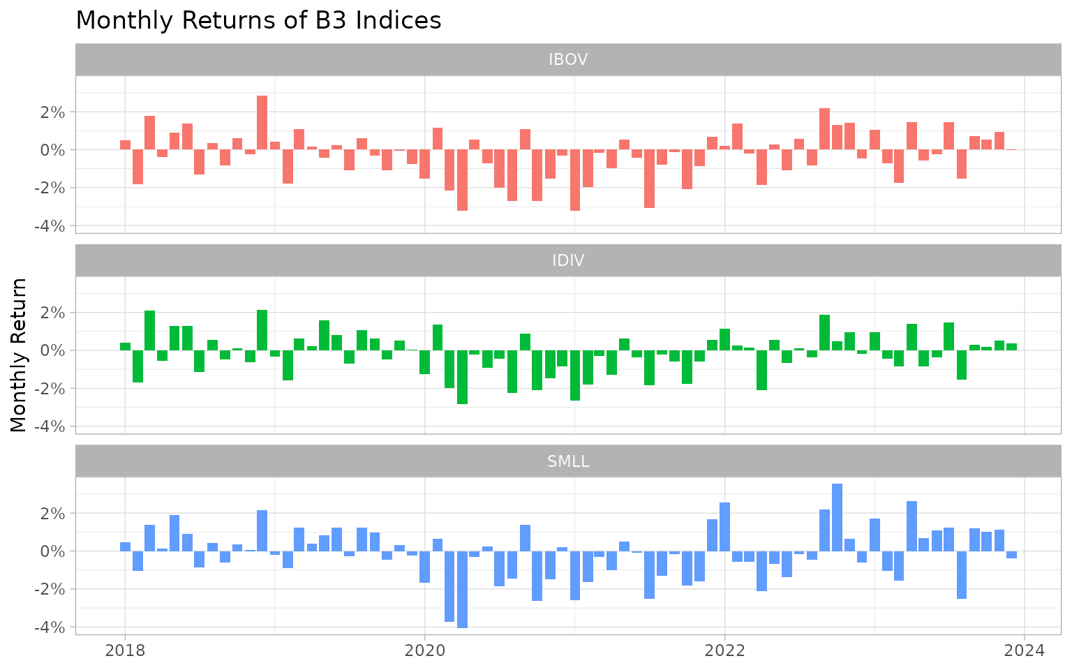

Monthly Returns of B3 Indices

Calculating summary statistics

You can calculate summary statistics to compare the performance of different indices:

# Calculate annualized summary statistics
performance_summary <- monthly_returns |>
  group_by(symbol) |>
  summarise(
    Mean = mean(monthly_return, na.rm = TRUE),
    Median = median(monthly_return, na.rm = TRUE),
    Std.Dev = sd(monthly_return, na.rm = TRUE),
    Min = min(monthly_return, na.rm = TRUE),
    Max = max(monthly_return, na.rm = TRUE),
    Positive = mean(monthly_return > 0, na.rm = TRUE)
  ) |>
  mutate(
    Annualized.Return = (1 + Mean)^12 - 1,
    Annualized.Volatility = Std.Dev * sqrt(12),
    Sharpe = Annualized.Return / Annualized.Volatility
  )

# Display the summary statistics
performance_summary |>
  select(symbol, Annualized.Return, Annualized.Volatility, Sharpe, Positive) |>
  mutate(
    Annualized.Return = scales::percent(Annualized.Return, accuracy = 0.01),
    Annualized.Volatility = scales::percent(Annualized.Volatility, accuracy = 0.01),
    Sharpe = round(Sharpe, 2),
    Positive = scales::percent(Positive, accuracy = 0.1)
  ) |>
  rename(
    Index = symbol,
    `Ann. Return` = Annualized.Return,
    `Ann. Volatility` = Annualized.Volatility,
    `Sharpe Ratio` = Sharpe,
    `% Positive Months` = Positive
  )
#> # A tibble: 3 × 5
#>   Index `Ann. Return` `Ann. Volatility` `Sharpe Ratio` `% Positive Months`
#>   <chr> <chr>         <chr>                      <dbl> <chr>              
#> 1 IBOV  -3.54%        4.60%                      -0.77 41.7%              
#> 2 IDIV  -2.18%        4.01%                      -0.55 47.2%              
#> 3 SMLL  -1.45%        5.17%                      -0.28 47.2%

Conclusion

This vignette demonstrated how to work with B3 index data using the rb3 package. We covered:

Retrieving Available Indices: Using indexes_get() to list all available B3 indices.
Historical Performance Analysis: Using b3-indexes-historical-data to analyze and visualize index performance over time.
Index Composition Analysis: Using b3-indexes-composition to understand which stocks belong to each index.
Portfolio Weight Analysis: Using b3-indexes-theoretical-portfolio to analyze the weights and concentration of indices.
Sector Exposure Analysis: Using b3-indexes-current-portfolio to analyze sector allocation within indices.
Performance Metrics: Calculating and comparing performance statistics across different indices.

The combination of these four templates provides a comprehensive toolkit for analyzing the Brazilian equity market through its indices, suitable for investors, researchers, and analysts.

For more advanced analyses, you might consider:

Tracking changes in index composition over time
Building factor models using index constituents
Creating custom indices based on specific criteria
Analyzing the relationship between index performance and macroeconomic variables
Constructing optimized portfolios based on index data