Accumulated Cyclone Energy (ACE)

library(dplyr)
library(ggplot2)
library(HURDAT)
library(lubridate)
library(readr)
library(rrricanes)
library(rrricanesdata)

ACE or Accumulated Cyclone Energy is a method of measuring energy of a cyclone or for an entire season. It is calculated by the formula

\[ \text{ACE} = 10^{-4}\sum{v^2_\text{max}} \]

where \(v_\text{max}\) is the wind speed in knots. Values may only be used when a storm is a tropical system with winds of at least 35 knots. Additionally, only six-hour intervals are used.

To calculate ACE you would want to use the fstadv dataset and apply the following rules:

since forecast/advisory products are typically issued at 03:00, 09:00, 15:00 and 21:00 UTC filter out odd hours
Status is Tropical Storm or Hurricane.
Wind is not NA
group by Key
select Wind

fstadv <- fstadv %>% 
    filter(hour(Date) %in% c(3, 9, 15, 21), 
           Status %in% c("Tropical Storm", "Hurricane"), 
           !is.na(Wind)) %>% 
    group_by(Key) %>% 
    select(Name, Wind)

## Adding missing grouping variables: `Key`

Now let’s summarise our dataset with new variable ACE.

fstadv %>% 
    summarise(Name = last(Name), 
              ACE = sum(Wind^2) * 1e-04) %>% 
    arrange(desc(ACE)) %>% 
    top_n(10)

## Selecting by ACE

## # A tibble: 10 x 3
##    Key      Name      ACE
##    <chr>    <chr>   <dbl>
##  1 AL092004 Ivan     69.9
##  2 AL112017 Irma     66.6
##  3 AL132003 Isabel   62.5
##  4 AL142016 Matthew  48.0
##  5 AL062004 Frances  46.9
##  6 AL152017 Maria    44.6
##  7 AL091999 Gert     44.0
##  8 AL112010 Igor     42.9
##  9 AL102003 Fabian   42.6
## 10 EP071999 Dora     42.2

This matches somewhat well with Wikipedia and other sources. But, you may notice we’re missing some storms. rrricanes currently only holds data back to 1998; this data is considered “real-time”.

A companion package, HURDAT is available in CRAN that has data for all cyclones dating back as far as 1851. This package has less data than rrricanes. But, as it is based on a post-storm reanalysis project, the data is more accurate.

Let’s revisit the top 10 using HURDAT:

AL %>% 
    filter(hour(DateTime) %in% c(0, 6, 12, 18), 
           Status %in% c("TS", "HU"), 
           !is.na(Wind)) %>% 
    group_by(Key) %>% 
    summarise(Name = last(Name), 
              ACE = sum(Wind^2) * 1e-04) %>% 
    arrange(desc(ACE)) %>% 
    top_n(10)

## Selecting by ACE

## # A tibble: 10 x 3
##    Key      Name      ACE
##    <chr>    <chr>   <dbl>
##  1 AL031899 UNNAMED  73.6
##  2 AL091893 UNNAMED  63.5
##  3 AL141932 UNNAMED  59.8
##  4 AL041906 UNNAMED  56.0
##  5 AL031915 UNNAMED  41.3
##  6 AL041898 UNNAMED  40.1
##  7 AL061893 UNNAMED  39.8
##  8 AL061915 UNNAMED  37.7
##  9 AL061886 UNNAMED  37.1
## 10 AL021915 UNNAMED  36.9

A couple of things to notice here:

in HURDAT, the common times used are 00:00, 06:00, 12:00 and 18:00 UTC
Our list is more comprehensive than the Wikipedia list as that list only measures storms after 1950.

ACE is slightly higher and that could be for a number of reasons. For example, on re-analysis the Hurricane Research Division may have determined a cyclone was actually tropical (shown in HURDAT) when initially it was believed to be extratropical (as shown in rrricanes). Or, and more likely, they determined through additional data that a storm was actually stronger than originally though.

You can also calculate ACE for a season. Instead of grouping by Key we group by Year. I’ll stick with HURDAT in this example.

(df <- AL %>% 
    mutate(Year = year(DateTime)) %>% 
    filter(hour(DateTime) %in% c(0, 6, 12, 18), 
           Status %in% c("TS", "HU"), 
           !is.na(Wind)) %>% 
    group_by(Year) %>% 
    summarise(ACE = sum(Wind^2) * 1e-04) %>% 
    arrange(desc(ACE))) %>% 
    top_n(10)

## Selecting by ACE

## # A tibble: 10 x 2
##     Year   ACE
##    <dbl> <dbl>
##  1  1893  231.
##  2  1887  181.
##  3  1886  166.
##  4  1906  163.
##  5  1899  151.
##  6  1916  144.
##  7  1896  136.
##  8  1894  135.
##  9  1915  130.
## 10  1891  116.

This also matches relatively well with that on Wikipedia and other sources.

ggplot(df, aes(x = Year, y = ACE)) + 
    geom_bar(stat = "identity") + 
    theme_bw()

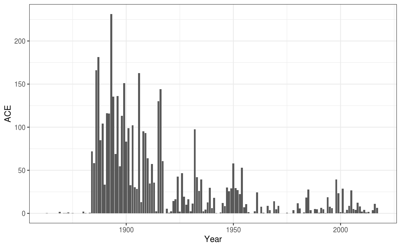
It would certainly seem that tropical cyclone activity ebbs and flows over time.

Tim Trice

June 27, 2017