Transition towards Open Access

Following the template in OpenAlex’s oa-percentage tutorial, this vignette uses openalexR to answer:

How many of recent journal articles from the University of Pennsylvania are open access? And how many aren’t?

library(openalexR)
library(dplyr)
library(tidyr)
library(ggplot2)

We first need to find the openalex.id for University of Pennsylvania. We can do this by fetching for the institutions entity and put “University of Pennsylvania” in display_name or display_name.search:

oa_fetch(
  entity = "inst", # same as "institutions"
  display_name.search = "\"University of Pennsylvania\""
) %>%
  select(display_name, ror) %>% 
  knitr::kable()

display_name	ror
University of Pennsylvania	https://ror.org/00b30xv10
Hospital of the University of Pennsylvania	https://ror.org/02917wp91
University of Pennsylvania Health System	https://ror.org/04h81rw26
Indiana University of Pennsylvania	https://ror.org/0511cmw96
California University of Pennsylvania	https://ror.org/01spssf70
Raymond and Ruth Perelman School of Medicine at the University of Pennsylvania	NA
Cheyney University of Pennsylvania	https://ror.org/02nckwn80

We will use the first ror, 00b30xv10, as one of the filters for our query.

Alternatively, we could go to the autocomplete endpoint at https://explore.openalex.org/ to search for “University of Pennsylvania” and find the ror there!

All other filters are straightforward and explained in detailed in the original jupyter notebook tutorial. The only difference here is that, instead of grouping by is_oa, we’re interested in the “trend” over the years, so we’re going to group by publication_year, and perform the query twice, one for is_oa = "true" and one for is_oa = "false" .

open_access <- oa_fetch(
  entity = "works",
  institutions.ror = "00b30xv10",
  type = "journal-article",
  from_publication_date = "2012-08-24",
  is_paratext = "false",
  is_oa = "true",
  group_by = "publication_year",
  count_only = TRUE
)

closed_access <- oa_fetch(
  entity = "works",
  institutions.ror = "00b30xv10",
  type = "journal-article",
  from_publication_date = "2012-08-24",
  is_paratext = "false",
  is_oa = "false",
  group_by = "publication_year",
  count_only = TRUE
)

uf_df <- closed_access %>%
  select(- key_display_name) %>%
  full_join(open_access, by = "key", suffix = c("_ca", "_oa")) 

uf_df
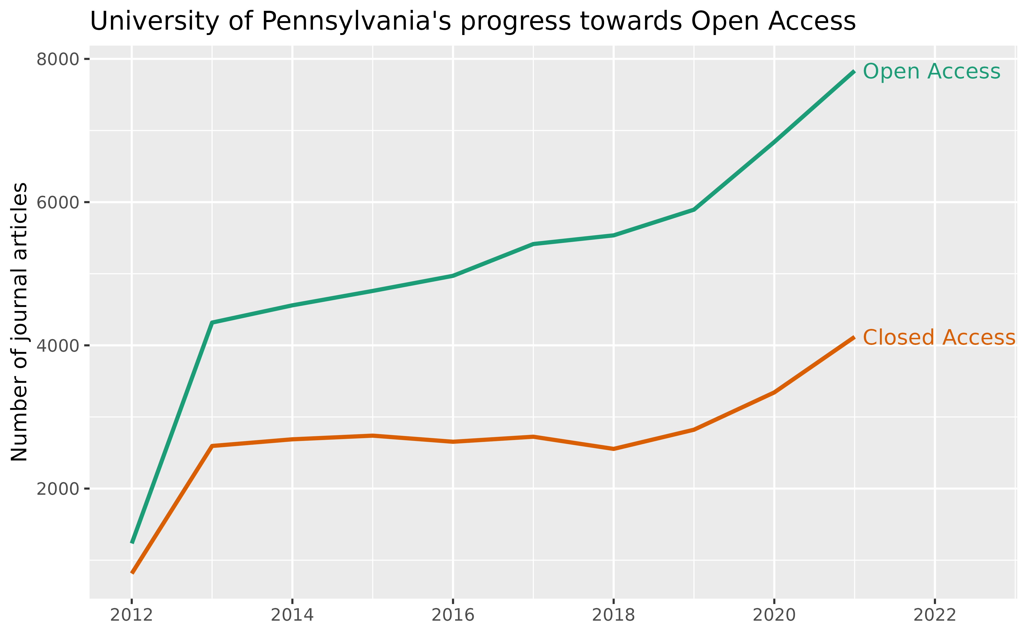
#>     key count_ca key_display_name count_oa
#> 1  2022     4280             2022     3997
#> 2  2021     4118             2021     7834
#> 3  2020     3343             2020     6840
#> 4  2019     2822             2019     5895
#> 5  2015     2739             2015     4760
#> 6  2017     2724             2017     5415
#> 7  2014     2688             2014     4559
#> 8  2016     2654             2016     4971
#> 9  2013     2595             2013     4318
#> 10 2018     2554             2018     5536
#> 11 2012      814             2012     1234
#> 12 2023      493             2023      433

Finally, we compare the number of open vs. closed access articles over the years:

uf_df %>%
  filter(key <= 2021) %>% # we do not yet have complete data for 2022 and after
  pivot_longer(cols = starts_with("count")) %>%
  mutate(
    year = as.integer(key),
    is_oa = recode(
      name,
      "count_ca" = "Closed Access",
      "count_oa" = "Open Access"
    ),
    label = if_else(key < 2021, NA_character_, is_oa)
  ) %>% 
  select(year, value, is_oa, label) %>%
  ggplot(aes(x = year, y = value, group = is_oa, color = is_oa)) +
  geom_line(size = 1) +
  labs(
    title = "University of Pennsylvania's progress towards Open Access",
    x = NULL, y = "Number of journal articles") +
  scale_color_brewer(palette = "Dark2", direction = -1) +
  scale_x_continuous(breaks = seq(2010, 2024, 2)) +
  geom_text(aes(label = label), nudge_x = 0.1, hjust = 0) +
  coord_cartesian(xlim = c(NA, 2022.5)) +
  guides(color = "none")