##
## Attaching package: 'dplyr'
## The following objects are masked from 'package:stats':
##
##     filter, lag
## The following objects are masked from 'package:base':
##
##     intersect, setdiff, setequal, union
## Linking to GEOS 3.10.2, GDAL 3.4.1, PROJ 8.2.1; sf_use_s2() is TRUE
## terra 1.7.78
##
## Attaching package: 'igraph'
## The following objects are masked from 'package:terra':
##
##     blocks, compare, union
## The following objects are masked from 'package:dplyr':
##
##     as_data_frame, groups, union
## The following objects are masked from 'package:stats':
##
##     decompose, spectrum
## The following object is masked from 'package:base':
##
##     union
##
## Attaching package: 'future'
## The following objects are masked from 'package:igraph':
##
##     %->%, %<-%
Computational grids
- Computational grids refer to a set of polygons that cover the entire
spatial domain of interest. These grids are used to split the spatial
domain into smaller pieces for parallel processing.
-
chopin provides functions to generate computational
grids for parallel processing by par_grid() function.
- The standard sequence of running
par_grid() includes
the following steps:
- Generate computational grids with
par_pad_grid() or
par_pad_balanced(). This step will give you a set of grid
polygons, one of which is original splits and the other is padded in
consideration of buffer radius in the subsequent spatial
operations.
- Run
par_grid() with the input dataset and the grid
polygons.
- Before advancing, we define terms for clarity.
-
Input data: the data where the computed value will
be stored. For example, when extracting raster values with vector
objects, vector objects are the input data.
-
Target data: the data from which the
values come. In the example above, raster object is the target
data.
- Original and padded grids will be used to split the main input with
the original grid and the target dataset for computation with the padded
grid, respectively.
Types of computational grids and their generation
- There are two approaches to generate computational grids. One is to
use
par_pad_grid() with one of three modes and
the other is to use par_group_grid(). Thus, users have
four options in total to generate computational
grids.
-
padding argument is very important to ensure the
accurate parallel operations in a case where buffering is involved.
Suppose a user has point geometry inputs and apply circular buffer with
a certain radius. Since the original grid (without padding = no overlap
between adjacent grids) filters the original input in each parallel
worker, points near each grid border may miss target data as buffered
polygons exceed the grid.
par_pad_grid(): standard interface
-
par_pad_grid() generates regular grid polygons with
padding for parallel processing. Padding is the distance of overlapping
between grid polygons, essentially from the buffer radius of the points
when buffer polygons are concerned.
-
par_pad_grid() supports three internal
modes:
-
mode = "grid": generates regular grid polygons with
padding, nx and ny arguments determine the
number of columns and rows in the grid, respectively.
-
mode = "grid_quantile": generates regular grid polygons
with padding based on quantiles of the number of points in each grid.
The grids will look irregular and the points per grid will be more
balanced than the grid mode.
-
mode = "grid_advanced": generates regular grid polygons
with padding based on the number of points in each grid and the number
of points in the entire dataset. nx and ny
arguments determine the number of columns and rows in the grid, then
merge_max argument controls how many adjacent grids are
merged into one grid. grid_min_features argument determines
the minimum number of points in each grid, which means grids with fewer
points than this value will be merged with adjacent grids. Adjusting
these arguments can balance the computational load among the threads and
reduce the overhead of parallelization.
par_pad_balanced(): focusing on getting the balanced
clusters
-
par_pad_balanced() groups the inputs into equal size,
then generates padded rectangles that cover the same number of points
per grid. Users can use the output of this function into
par_grid() for parallel processing.
Random points in NC
- For demonstration of
par_pad_grid(), we use moderately
clustered point locations generated inside the counties of North
Carolina.

## Loading required package: spatstat.data
## Loading required package: spatstat.univar
## spatstat.univar 3.0-1
## Loading required package: spatstat.geom
## spatstat.geom 3.3-2
##
## Attaching package: 'spatstat.geom'
## The following objects are masked from 'package:igraph':
##
##     diameter, edges, is.connected, vertices
## The following objects are masked from 'package:terra':
##
##     area, delaunay, is.empty, rescale, rotate, shift, where.max,
##     where.min
## spatstat.random 3.3-1

# convert to terra SpatVector
ncpoints_tr <- terra::vect(ncpoints)
Visualize computational grids
- The output of
par_pad_grid() and
par_pad_balanced() is length 2 list. A significant
difference between the two is the first element of the output. In
par_pad_grid(), it is always a sf or SpatVector object with
polygon geometries. On the other hand, par_pad_balanced()
will have the first element as a sf or SpatVector object with the same
geometry type as the original input. For example, it will have point
geometries if the input was point.
compregions <-
  chopin::par_pad_grid(
    ncpoints_tr,
    mode = "grid",
    nx = 8L,
    ny = 5L,
    padding = 1e4L
  )

# a list object
class(compregions)
## [1] "list"
# length of 2
names(compregions)
## [1] "original" "padded"
par(mfrow = c(2, 1))
plot(compregions$original, main = "Original grids")
plot(compregions$padded, main = "Padded grids")

Generate regular grid computational regions
-
chopin::par_pad_grid() takes a spatial dataset to
generate regular grid polygons with nx and ny
arguments with padding. Users will have both overlapping (by the degree
of radius) and non-overlapping grids, both of which will be
utilized to split locations and target datasets into sub-datasets for
efficient processing.
compregions <-
  chopin::par_pad_grid(
    ncpoints_tr,
    mode = "grid",
    nx = 8L,
    ny = 5L,
    padding = 1e4L
  )
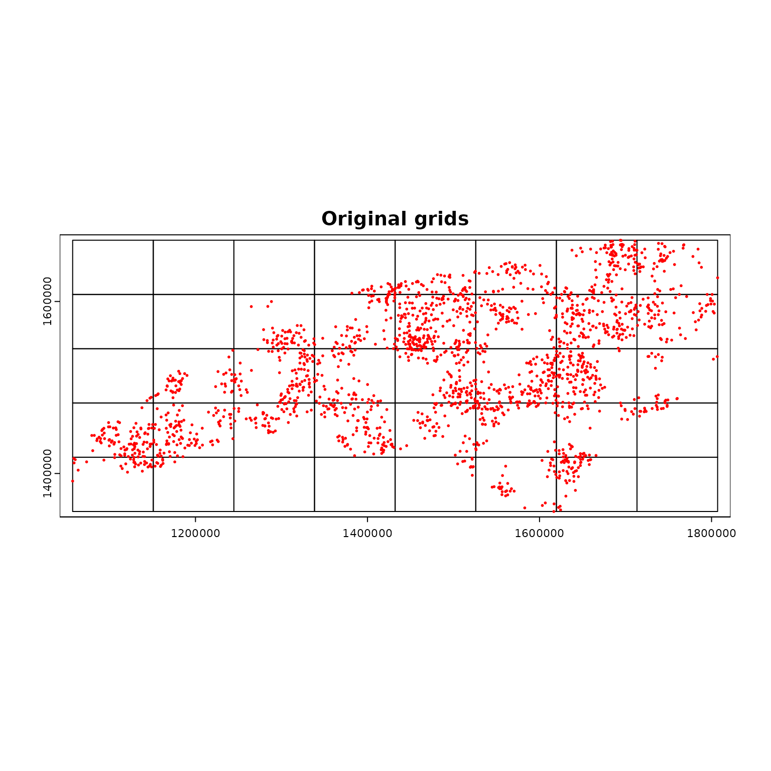
- The output of
par_pad_grid() is a list object with two
elements named original (non-overlapping grid polygons) and
padded (overlapping by padding). The class of
each element depends on the input dataset class. The figures below
illustrate the grid polygons with and without overlaps.
## [1] "original" "padded"
oldpar <- par()
par(mfrow = c(2, 1))
terra::plot(compregions$original, main = "Original grids")
terra::plot(compregions$padded, main = "Padded grids")

par(mfrow = c(1, 1))
terra::plot(compregions$original, main = "Original grids")
terra::plot(ncpoints_tr, add = TRUE, col = "red", cex = 0.4)

Split the points by two 1D quantiles
-
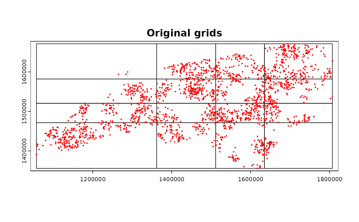
mode = "grid_quantile" generates regular grid polygons
with padding based on quantiles of the coordinates in each
dimension.
- When using this mode, users should define
quantiles
argument, which will be used to get the same number of quantiles in each
dimension. A convenient way to define seq() function with
length.out argument. The example below uses
length.out = 5, which will give quartiles.
grid_quantiles <-
  chopin::par_pad_grid(
    input = ncpoints_tr,
    mode = "grid_quantile",
    quantiles = seq(0, 1, length.out = 5),
    padding = 1e4L
  )

names(grid_quantiles)
## [1] "original" "padded"
par(mfrow = c(2, 1))
terra::plot(grid_quantiles$original, main = "Original grids")
terra::plot(grid_quantiles$padded, main = "Padded grids")

par(mfrow = c(1, 1))
terra::plot(grid_quantiles$original, main = "Original grids")
terra::plot(ncpoints_tr, add = TRUE, col = "red", cex = 0.4)

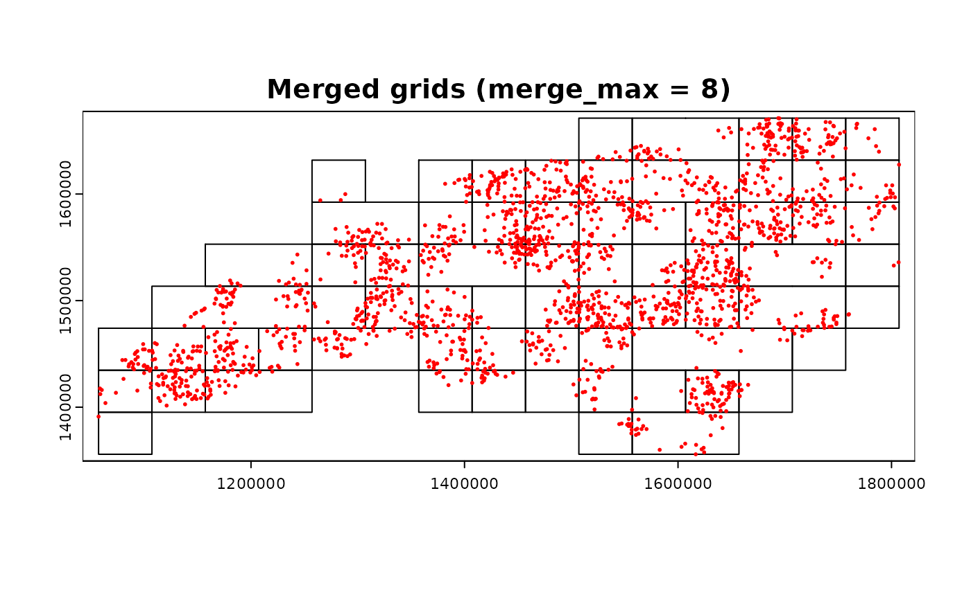
Merge the grids based on the number of points
-
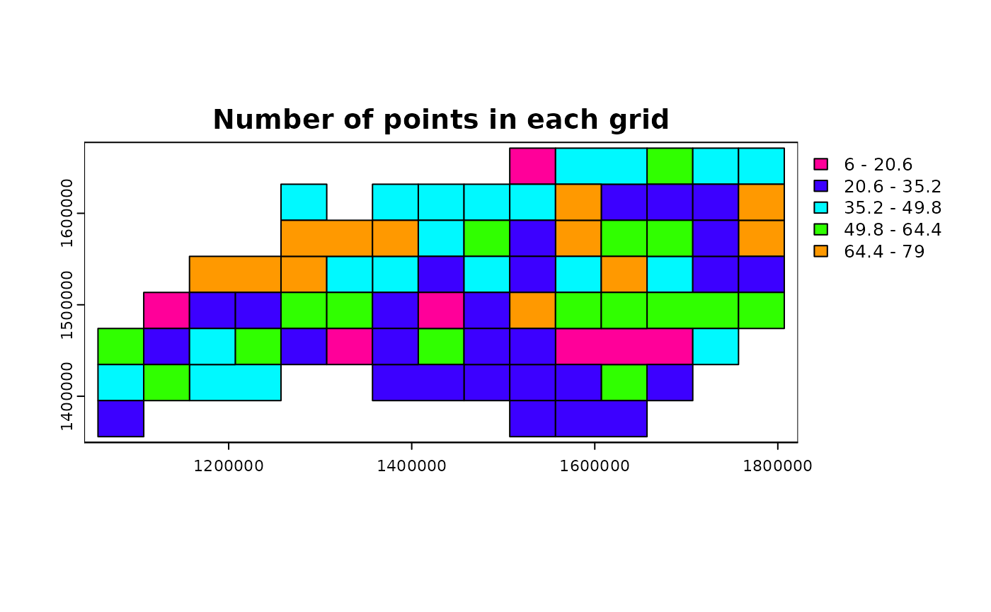
mode = "grid_advanced" utilizes finer grids to merge
the results from the finer grids into the coarser grids. This behavior
can balance the computational load among the threads and reduce the
overhead of parallelization. That said, this mode internally generates
grids in mode = "grid" and merges them based on the number
of points in each grid.
- To determine the adjacency and merging behavior, minimum spanning
tree (MST) is identified. The function utilizes
igraph::mst() for MST identification and other graph
summary functions under the hood.
- As a note, users can adjust the merging behavior by changing the
arguments
grid_min_features and
merge_max.
grid_advanced1 <-
  chopin::par_pad_grid(
    input = ncpoints_tr,
    mode = "grid_advanced",
    nx = 15L,
    ny = 8L,
    padding = 1e4L,
    grid_min_features = 25L,
    merge_max = 5L
  )
## Switch terra class to sf...
## Switch terra class to sf...
## ℹ The merged polygons have too complex shapes.
## Increase threshold or use the original grids.
##
## Switch sf class to terra...
par(mfrow = c(2, 1))
terra::plot(grid_advanced1$original, main = "Original grids")
terra::plot(grid_advanced1$padded, main = "Padded grids")

par(mfrow = c(1, 1))
terra::plot(grid_advanced1$original, main = "Merged grids (merge_max = 5)")
terra::plot(ncpoints_tr, add = TRUE, col = "red", cex = 0.4)

ncpoints_tr$n <- 1
n_points <-
  terra::zonal(
    ncpoints_tr,
    grid_advanced1$original,
    fun = "sum"
  )[["n"]]

grid_advanced1g <- grid_advanced1$original
grid_advanced1g$n_points <- n_points

terra::plot(grid_advanced1g, "n_points", main = "Number of points in each grid")

Different values in merge_max
- Keeping other arguments the same, we can see the difference in the
number of merged grids by changing the
merge_max
argument.
grid_advanced2 <-
  chopin::par_pad_grid(
    input = ncpoints_tr,
    mode = "grid_advanced",
    nx = 15L,
    ny = 8L,
    padding = 1e4L,
    grid_min_features = 30L,
    merge_max = 4L
  )
## Switch terra class to sf...
## Switch terra class to sf...
## ℹ The merged polygons have too complex shapes.
## Increase threshold or use the original grids.
##
## Switch sf class to terra...
par(mfrow = c(2, 1))
terra::plot(grid_advanced2$original, main = "Original grids")
terra::plot(grid_advanced2$padded, main = "Padded grids")

par(mfrow = c(1, 1))
terra::plot(grid_advanced2$original, main = "Merged grids (merge_max = 8)")
terra::plot(ncpoints_tr, add = TRUE, col = "red", cex = 0.4)

grid_advanced3 <-
  chopin::par_pad_grid(
    input = ncpoints_tr,
    mode = "grid_advanced",
    nx = 15L,
    ny = 8L,
    padding = 1e4L,
    grid_min_features = 25L,
    merge_max = 3L
  )
## Switch terra class to sf...
## Switch terra class to sf...
## ℹ The merged polygons have too complex shapes.
## Increase threshold or use the original grids.
##
## Switch sf class to terra...
par(mfrow = c(2, 1))
terra::plot(grid_advanced3$original, main = "Original grids")
terra::plot(grid_advanced3$padded, main = "Padded grids")

par(mfrow = c(1, 1))
terra::plot(grid_advanced3$original, main = "Merged grids (merge_max = 3)")
terra::plot(ncpoints_tr, add = TRUE, col = "red", cex = 0.4)

par_make_balanced()
-
par_make_balanced() uses anticlust package
to split the point set into the balanced clusters.
- In the background,
par_pad_balanced() is run first to
generate the equally sized clusters from the input. Then, padding is
applied to the extent of each cluster to be compatible with
par_grid(), where both the original and the padded grids
are used.
- Please note that
ngroups argument value must be the
exact divisor of the number of points. For example, in
the example below, when one changes ngroups to
10L, it will fail as the number of points is not divisible
by 10.
- Consult the
anticlust
package for more details on the algorithm.
-
par_pad_balanced() makes a compatible object to the
output of par_pad_grid() directly from the input
points.
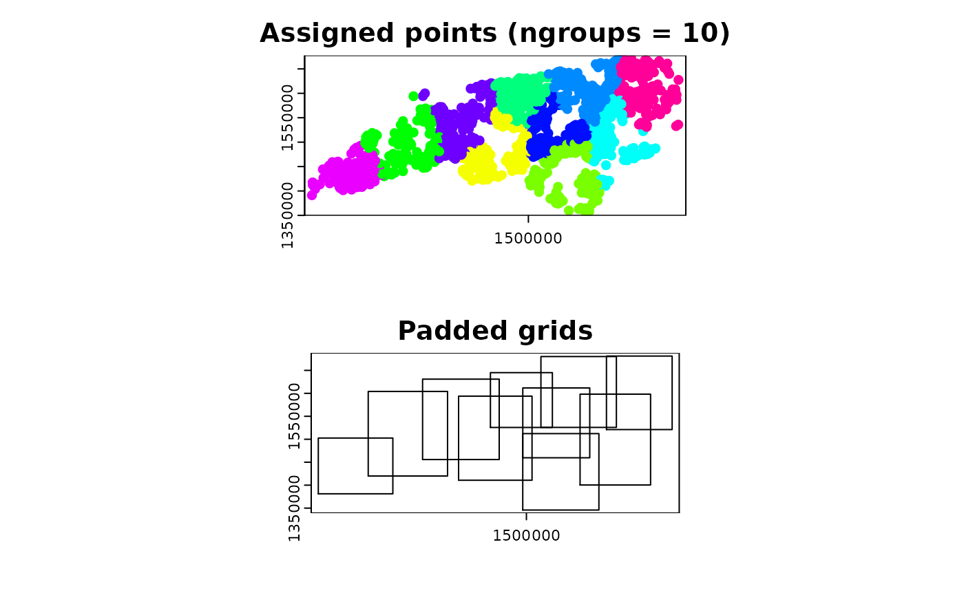
- As illustrated in the figure below, the points will be split into
ngroups clusters with the same number of points then
processed in parallel by using the output object with
par_grid().
# ngroups should be the exact divisor of the number of points!
group_bal_grid <-
  chopin::par_pad_balanced(
    points_in = ncpoints_tr,
    ngroups = 10L,
    padding = 1e4
  )
group_bal_grid$original$CGRIDID <- as.factor(group_bal_grid$original$CGRIDID)

par(mfrow = c(2, 1))
terra::plot(group_bal_grid$original, "CGRIDID",
            legend = FALSE,
            main = "Assigned points (ngroups = 10)")
terra::plot(group_bal_grid$padded, main = "Padded grids")
