rnoaa tutorial
for v0.5.2
## Installation
Install and load `rnoaa` into the R session. Stable version from CRAN
```r
install.packages("rnoaa")
```
Or development version from Github:
```r
install.packages("devtools")
devtools::install_github("ropensci/rnoaa")
```
```r
library('plyr')
library('rnoaa')
```
## Usage
## National Climatic Data Center (NCDC) data
### Get info on a station by specifying a datasetid, locationid, and stationid
```r
ncdc_stations(datasetid='GHCND', locationid='FIPS:12017', stationid='GHCND:USC00084289')
```
```
#> $meta
#> NULL
#>
#> $data
#> elevation mindate maxdate latitude name
#> 1 12.2 1899-02-01 2016-04-30 28.8029 INVERNESS 3 SE, FL US
#> datacoverage id elevationUnit longitude
#> 1 1 GHCND:USC00084289 METERS -82.3126
#>
#> attr(,"class")
#> [1] "ncdc_stations"
```
### Search for data and get a data.frame
```r
out <- ncdc(datasetid='NORMAL_DLY', datatypeid='dly-tmax-normal', startdate = '2010-05-01', enddate = '2010-05-10')
```
See a data.frame
```r
out$data
```
```
#> date datatype station value fl_c
#> 1 2010-05-01T00:00:00 DLY-TMAX-NORMAL GHCND:AQW00061705 869 C
#> 2 2010-05-01T00:00:00 DLY-TMAX-NORMAL GHCND:CAW00064757 607 Q
#> 3 2010-05-01T00:00:00 DLY-TMAX-NORMAL GHCND:CQC00914080 840 R
#> 4 2010-05-01T00:00:00 DLY-TMAX-NORMAL GHCND:CQC00914801 858 R
#> 5 2010-05-01T00:00:00 DLY-TMAX-NORMAL GHCND:FMC00914395 876 P
#> 6 2010-05-01T00:00:00 DLY-TMAX-NORMAL GHCND:FMC00914419 885 P
#> 7 2010-05-01T00:00:00 DLY-TMAX-NORMAL GHCND:FMC00914446 885 P
#> 8 2010-05-01T00:00:00 DLY-TMAX-NORMAL GHCND:FMC00914482 868 R
#> 9 2010-05-01T00:00:00 DLY-TMAX-NORMAL GHCND:FMC00914720 899 R
#> 10 2010-05-01T00:00:00 DLY-TMAX-NORMAL GHCND:FMC00914761 897 P
#> 11 2010-05-01T00:00:00 DLY-TMAX-NORMAL GHCND:FMC00914831 870 P
#> 12 2010-05-01T00:00:00 DLY-TMAX-NORMAL GHCND:FMC00914892 883 P
#> 13 2010-05-01T00:00:00 DLY-TMAX-NORMAL GHCND:FMC00914898 875 P
#> 14 2010-05-01T00:00:00 DLY-TMAX-NORMAL GHCND:FMC00914911 885 P
#> 15 2010-05-01T00:00:00 DLY-TMAX-NORMAL GHCND:FMW00040308 888 S
#> 16 2010-05-01T00:00:00 DLY-TMAX-NORMAL GHCND:FMW00040504 879 C
#> 17 2010-05-01T00:00:00 DLY-TMAX-NORMAL GHCND:FMW00040505 867 S
#> 18 2010-05-01T00:00:00 DLY-TMAX-NORMAL GHCND:GQC00914025 852 P
#> 19 2010-05-01T00:00:00 DLY-TMAX-NORMAL GHCND:GQW00041415 877 C
#> 20 2010-05-01T00:00:00 DLY-TMAX-NORMAL GHCND:JQW00021603 852 P
#> 21 2010-05-01T00:00:00 DLY-TMAX-NORMAL GHCND:PSC00914519 883 P
#> 22 2010-05-01T00:00:00 DLY-TMAX-NORMAL GHCND:PSC00914712 840 P
#> 23 2010-05-01T00:00:00 DLY-TMAX-NORMAL GHCND:PSW00040309 879 S
#> 24 2010-05-01T00:00:00 DLY-TMAX-NORMAL GHCND:RMW00040604 867 S
#> 25 2010-05-01T00:00:00 DLY-TMAX-NORMAL GHCND:RMW00040710 863 C
```
### Plot data, super simple, but it's a start
```r
out <- ncdc(datasetid='NORMAL_DLY', stationid='GHCND:USW00014895', datatypeid='dly-tmax-normal', startdate = '2010-01-01', enddate = '2010-12-10', limit = 300)
ncdc_plot(out)
```
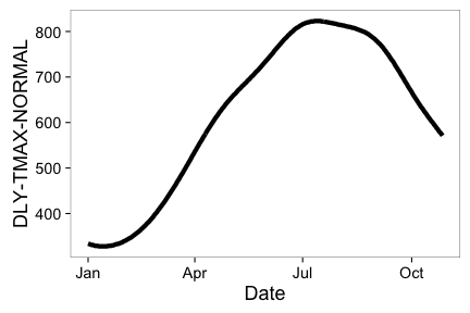
Note that the x-axis tick text is not readable, but see futher down in tutorial for how to adjust that.
### More on plotting
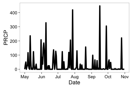
#### Example 1
Search for data first, then plot
```r
out <- ncdc(datasetid='GHCND', stationid='GHCND:USW00014895', datatypeid='PRCP', startdate = '2010-05-01', enddate = '2010-10-31', limit=500)
```
Default plot
```r
ncdc_plot(out)
```
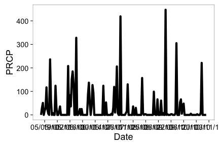
Create 14 day breaks
```r
ncdc_plot(out, breaks="14 days")
```
```
#> Error: Invalid input: time_trans works with objects of class POSIXct only
```
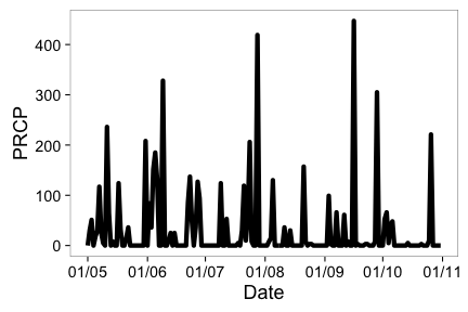
One month breaks
```r
ncdc_plot(out, breaks="1 month", dateformat="%d/%m")
```
```
#> Error: Invalid input: time_trans works with objects of class POSIXct only
```
#### Example 2
Search for data
```r
out2 <- ncdc(datasetid='GHCND', stationid='GHCND:USW00014895', datatypeid='PRCP', startdate = '2010-05-01', enddate = '2010-05-03', limit=100)
```
Make a plot, with 6 hour breaks, and date format with only hour
```r
ncdc_plot(out2, breaks="6 hours", dateformat="%H")
```
```
#> Error: Invalid input: time_trans works with objects of class POSIXct only
```
### Combine many calls to noaa function
Search for two sets of data
```r
out1 <- ncdc(datasetid='GHCND', stationid='GHCND:USW00014895', datatypeid='PRCP', startdate = '2010-03-01', enddate = '2010-05-31', limit=500)
out2 <- ncdc(datasetid='GHCND', stationid='GHCND:USW00014895', datatypeid='PRCP', startdate = '2010-09-01', enddate = '2010-10-31', limit=500)
```
Then combine with a call to `ncdc_combine`
```r
df <- ncdc_combine(out1, out2)
head(df[[1]]); tail(df[[1]])
```
```
#> date datatype station value fl_m fl_q fl_so
#> 1 2010-03-01T00:00:00 PRCP GHCND:USW00014895 0 T 0
#> 2 2010-03-02T00:00:00 PRCP GHCND:USW00014895 0 T 0
#> 3 2010-03-03T00:00:00 PRCP GHCND:USW00014895 0 T 0
#> 4 2010-03-04T00:00:00 PRCP GHCND:USW00014895 0 0
#> 5 2010-03-05T00:00:00 PRCP GHCND:USW00014895 0 0
#> 6 2010-03-06T00:00:00 PRCP GHCND:USW00014895 0 0
#> fl_t
#> 1 2400
#> 2 2400
#> 3 2400
#> 4 2400
#> 5 2400
#> 6 2400
```
```
#> date datatype station value fl_m fl_q fl_so
#> 148 2010-10-26T00:00:00 PRCP GHCND:USW00014895 221 0
#> 149 2010-10-27T00:00:00 PRCP GHCND:USW00014895 0 0
#> 150 2010-10-28T00:00:00 PRCP GHCND:USW00014895 0 T 0
#> 151 2010-10-29T00:00:00 PRCP GHCND:USW00014895 0 T 0
#> 152 2010-10-30T00:00:00 PRCP GHCND:USW00014895 0 0
#> 153 2010-10-31T00:00:00 PRCP GHCND:USW00014895 0 0
#> fl_t
#> 148 2400
#> 149 2400
#> 150 2400
#> 151 2400
#> 152 2400
#> 153 2400
```
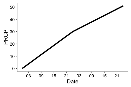
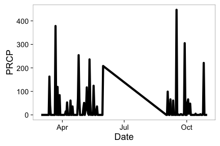
Then plot - the default passing in the combined plot plots the data together. In this case it looks kind of weird since a straight line combines two distant dates.
```r
ncdc_plot(df)
```
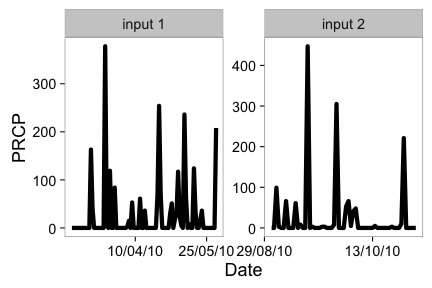
But we can pass in each separately, which uses `facet_wrap` in `ggplot2` to plot each set of data in its own panel.
```r
ncdc_plot(out1, out2, breaks="45 days")
```
```
#> Error: Invalid input: time_trans works with objects of class POSIXct only
```
## ERDDAP data
> ERDDAP data is now avialable through the `rerddap` package
## Severe Weather Data Inventory (SWDI) data
### Search for nx3tvs data from 5 May 2006 to 6 May 2006
```r
swdi(dataset='nx3tvs', startdate='20060505', enddate='20060506')
```
```
#> $meta
#> $meta$totalCount
#> numeric(0)
#>
#> $meta$totalTimeInSeconds
#> [1] 0.038
#>
#>
#> $data
#> ztime wsr_id cell_id cell_type range azimuth max_shear
#> 1 2006-05-05T00:05:50Z KBMX Q0 TVS 7 217 403
#> 2 2006-05-05T00:10:02Z KBMX Q0 TVS 5 208 421
#> 3 2006-05-05T00:12:34Z KSJT P2 TVS 49 106 17
#> 4 2006-05-05T00:17:31Z KSJT B4 TVS 40 297 25
#> 5 2006-05-05T00:29:13Z KMAF H4 TVS 53 333 34
#> 6 2006-05-05T00:31:25Z KLBB N0 TVS 51 241 24
#> 7 2006-05-05T00:33:25Z KMAF H4 TVS 52 334 46
#> 8 2006-05-05T00:37:37Z KMAF H4 TVS 50 334 34
#> 9 2006-05-05T00:41:51Z KMAF H4 TVS 51 335 29
#> 10 2006-05-05T00:44:33Z KLBB N0 TVS 46 245 35
#> 11 2006-05-05T00:46:03Z KMAF H4 TVS 49 335 41
#> 12 2006-05-05T00:48:55Z KLBB N0 TVS 44 246 44
#> 13 2006-05-05T00:50:16Z KMAF H4 TVS 49 337 33
#> 14 2006-05-05T00:54:29Z KMAF H4 TVS 47 337 42
#> 15 2006-05-05T00:57:42Z KLBB N0 TVS 41 251 46
#> 16 2006-05-05T00:58:41Z KMAF H4 TVS 46 340 29
#> 17 2006-05-05T01:02:04Z KLBB N0 TVS 39 251 42
#> 18 2006-05-05T01:02:53Z KMAF H4 TVS 46 339 35
#> 19 2006-05-05T01:02:53Z KMAF H4 TVS 50 338 27
#> 20 2006-05-05T01:06:26Z KLBB N0 TVS 36 251 31
#> 21 2006-05-05T01:07:06Z KMAF F5 TVS 45 342 44
#> 22 2006-05-05T01:10:48Z KLBB N0 TVS 36 256 37
#> 23 2006-05-05T01:11:18Z KMAF F5 TVS 45 343 39
#> 24 2006-05-05T01:15:30Z KMAF F5 TVS 44 344 30
#> 25 2006-05-05T01:15:30Z KMAF H4 TVS 49 341 26
#> mxdv
#> 1 116
#> 2 120
#> 3 52
#> 4 62
#> 5 111
#> 6 78
#> 7 145
#> 8 107
#> 9 91
#> 10 100
#> 11 127
#> 12 121
#> 13 98
#> 14 126
#> 15 117
#> 16 85
#> 17 102
#> 18 101
#> 19 84
#> 20 70
#> 21 120
#> 22 83
#> 23 108
#> 24 78
#> 25 81
#>
#> $shape
#> shape
#> 1 POINT (-86.8535716274277 33.0786326913943)
#> 2 POINT (-86.8165772540846 33.0982820681588)
#> 3 POINT (-99.5771091971025 31.1421609654838)
#> 4 POINT (-101.188161700093 31.672392833416)
#> 5 POINT (-102.664426480293 32.7306917937698)
#> 6 POINT (-102.70047613441 33.2380072329615)
#> 7 POINT (-102.6393683028 32.7226656893341)
#> 8 POINT (-102.621904684258 32.6927081076156)
#> 9 POINT (-102.614794815627 32.714139844846)
#> 10 POINT (-102.643380529494 33.3266446067682)
#> 11 POINT (-102.597961935071 32.6839260102062)
#> 12 POINT (-102.613894688178 33.3526192273658)
#> 13 POINT (-102.567153417051 32.6956373348052)
#> 14 POINT (-102.551596970251 32.664939580306)
#> 15 POINT (-102.586119971014 33.4287323151248)
#> 16 POINT (-102.499638479193 32.6644438090742)
#> 17 POINT (-102.5485490063 33.4398330734778)
#> 18 POINT (-102.51446954228 32.6597119240996)
#> 19 POINT (-102.559031583693 32.7166090376869)
#> 20 POINT (-102.492174522228 33.4564626989719)
#> 21 POINT (-102.463540844324 32.6573739036181)
#> 22 POINT (-102.510349454162 33.5066366303981)
#> 23 POINT (-102.448763863447 32.6613484943994)
#> 24 POINT (-102.42842159557 32.649061124799)
#> 25 POINT (-102.504158884526 32.7162751126854)
#>
#> attr(,"class")
#> [1] "swdi"
```
### Use an id
```r
out <- swdi(dataset='warn', startdate='20060506', enddate='20060507', id=533623)
list(out$meta, head(out$data), head(out$shape))
```
```
#> [[1]]
#> [[1]]$totalCount
#> numeric(0)
#>
#> [[1]]$totalTimeInSeconds
#> [1] 0.475
#>
#>
#> [[2]]
#> ztime_start ztime_end id warningtype
#> 1 2006-05-05T22:53:00Z 2006-05-06T00:00:00Z 397428 SEVERE THUNDERSTORM
#> 2 2006-05-05T22:55:00Z 2006-05-06T00:00:00Z 397429 SEVERE THUNDERSTORM
#> 3 2006-05-05T22:55:00Z 2006-05-06T00:00:00Z 397430 SEVERE THUNDERSTORM
#> 4 2006-05-05T22:57:00Z 2006-05-06T00:00:00Z 397431 SEVERE THUNDERSTORM
#> 5 2006-05-05T23:03:00Z 2006-05-06T00:00:00Z 397434 SEVERE THUNDERSTORM
#> 6 2006-05-05T23:14:00Z 2006-05-06T00:15:00Z 397437 SEVERE THUNDERSTORM
#> issuewfo messageid
#> 1 KLCH 052252
#> 2 KLUB 052256
#> 3 KLUB 052256
#> 4 KMAF 052258
#> 5 KMAF 052305
#> 6 KLUB 052315
#>
#> [[3]]
#> shape
#> 1 POLYGON ((-93.27 30.38, -93.29 30.18, -93.02 30.18, -93.04 30.37, -93.27 30.38))
#> 2 POLYGON ((-101.93 34.74, -101.96 34.35, -101.48 34.42, -101.49 34.74, -101.93 34.74))
#> 3 POLYGON ((-100.36 33.03, -99.99 33.3, -99.99 33.39, -100.28 33.39, -100.5 33.18, -100.51 33.02, -100.45 32.97, -100.37 33.03, -100.36 33.03))
#> 4 POLYGON ((-102.8 30.74, -102.78 30.57, -102.15 30.61, -102.15 30.66, -101.92 30.68, -102.07 30.83, -102.8 30.74))
#> 5 POLYGON ((-103.02 32.94, -103.03 32.66, -102.21 32.53, -102.22 32.95, -103.02 32.94))
#> 6 POLYGON ((-101.6 33.32, -101.57 33.31, -101.57 33.51, -101.65 33.51, -101.66 33.5, -101.75 33.5, -101.77 33.49, -101.84 33.49, -101.84 33.32, -101.6 33.32))
```
### Get all 'plsr' within the bounding box (-91,30,-90,31)
```r
swdi(dataset='plsr', startdate='20060505', enddate='20060510', bbox=c(-91,30,-90,31))
```
```
#> $meta
#> $meta$totalCount
#> numeric(0)
#>
#> $meta$totalTimeInSeconds
#> [1] 0.001
#>
#>
#> $data
#> ztime id event magnitude city
#> 1 2006-05-09T02:20:00Z 427540 HAIL 1 5 E KENTWOOD
#> 2 2006-05-09T02:40:00Z 427536 HAIL 1 MOUNT HERMAN
#> 3 2006-05-09T02:40:00Z 427537 TSTM WND DMG -9999 MOUNT HERMAN
#> 4 2006-05-09T03:00:00Z 427199 HAIL 0 FRANKLINTON
#> 5 2006-05-09T03:17:00Z 427200 TORNADO -9999 5 S FRANKLINTON
#> county state source
#> 1 TANGIPAHOA LA TRAINED SPOTTER
#> 2 WASHINGTON LA TRAINED SPOTTER
#> 3 WASHINGTON LA TRAINED SPOTTER
#> 4 WASHINGTON LA AMATEUR RADIO
#> 5 WASHINGTON LA LAW ENFORCEMENT
#>
#> $shape
#> shape
#> 1 POINT (-90.43 30.93)
#> 2 POINT (-90.3 30.96)
#> 3 POINT (-90.3 30.96)
#> 4 POINT (-90.14 30.85)
#> 5 POINT (-90.14 30.78)
#>
#> attr(,"class")
#> [1] "swdi"
```
## Sea ice data
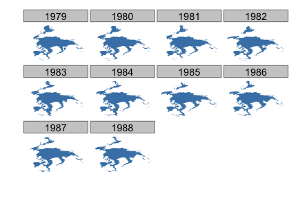
### Map all years for April only for North pole
```r
urls <- seaiceeurls(mo='Apr', pole='N')[1:10]
out <- lapply(urls, seaice)
names(out) <- seq(1979,1988,1)
df <- ldply(out)
library('ggplot2')
ggplot(df, aes(long, lat, group=group)) +
geom_polygon(fill="steelblue") +
theme_ice() +
facet_wrap(~ .id)
```
## IBTrACS storm data
Get NOAA wind storm tabular data, metadata, or shp files from International Best Track Archive for Climate Stewardship (IBTrACS). See http://www.ncdc.noaa.gov/ibtracs/index.php?name=numbering for more.
### Metadata
There are two datasets stored in the package. By default `storm_meta()` gives metadata describing columns of the datasets returned.
```r
head( storm_meta() )
```
```
#> Column_number Column_name units Shapefile_pt_flag
#> 1 1 Serial_Num N/A 1
#> 2 2 Season Year 1
#> 3 3 Num # 1
#> 4 4 Basin BB 1
#> 5 5 Sub_basin BB 1
#> 6 6 Name N/A 1
#> Shapefile_pt_attribute_name shapefile_att_type shapefile_att_len
#> 1 Serial_Num 7 13
#> 2 Season 3 4
#> 3 Num 3 5
#> 4 Basin 7 3
#> 5 Sub_basin 7 3
#> 6 Name 7 57
#> shapefile_att_prc
#> 1 0
#> 2 0
#> 3 0
#> 4 0
#> 5 0
#> 6 0
```
Or you can get back a dataset of storm names, including storm ids and their names.
```r
head( storm_meta("storm_names") )
```
```
#> id name
#> 1 1842298N11080 NOT NAMED(td9636)
#> 2 1845336N10074 NOT NAMED(td9636)
#> 3 1848011S09079 NOT NAMED(td9636)
#> 4 1848011S09080 XXXX848003(reunion)
#> 5 1848011S15057 XXXX848002(reunion)
#> 6 1848011S16057 NOT NAMED(td9636)
```
### Tabular data
You can get tabular data for basins, storms, or years, (or all data). `storm_data()` and the next function `storm_shp()` figure out what files to get, and gets them from an ftp server, and saves them to your machine. Do let us know if you have any problems with paths on your machine, and we'll fix 'em. The result from `storm_data()` is a `dplyr`-like data.frame with a easy summary that makes large datasets easy to view.
First, by basin (one of EP, NA, NI, SA, SI, SP, or WP)
```r
storm_data(year=1941)
#> ~/.rnoaa/storms/year/Year.1941.ibtracs_all.v03r06.csv
#>
#>
#> Size: 1766 X 195
#>
#> serial_num season num basin sub_basin name iso_time nature latitude
#> 1 1940215S18149 1941 1 SP EA NOT NAMED 1940-08-01 12:00:00 NR -999
#> 2 1940215S18149 1941 1 SP EA NOT NAMED 1940-08-01 18:00:00 NR -999
#> 3 1940215S18149 1941 1 SP EA NOT NAMED 1940-08-02 00:00:00 NR -999
#> 4 1940215S18149 1941 1 SP EA NOT NAMED 1940-08-02 06:00:00 NR -999
#> 5 1940215S18149 1941 1 SP EA NOT NAMED 1940-08-02 12:00:00 NR -999
#> 6 1940215S18149 1941 1 SP EA NOT NAMED 1940-08-02 18:00:00 NR -999
#> 7 1940215S18149 1941 1 SP EA NOT NAMED 1940-08-03 00:00:00 NR -999
#> 8 1940215S18149 1941 1 SP EA NOT NAMED 1940-08-03 06:00:00 NR -999
#> 9 1940215S18149 1941 1 SP EA NOT NAMED 1940-08-03 12:00:00 NR -999
#> 10 1940215S18149 1941 1 SP EA NOT NAMED 1940-08-03 18:00:00 NR -999
#> .. ... ... ... ... ... ... ... ... ...
#> Variables not shown: longitude (dbl), wind.wmo. (dbl), pres.wmo. (dbl), center (chr),
#> wind.wmo..percentile (dbl), pres.wmo..percentile (dbl), track_type (chr),
#> latitude_for_mapping (dbl), longitude_for_mapping (dbl), current.basin (chr), hurdat_atl_lat
#> (dbl), hurdat_atl_lon (dbl), hurdat_atl_grade (dbl), hurdat_atl_wind (dbl), hurdat_atl_pres
#> (dbl), td9636_lat (dbl), td9636_lon (dbl), td9636_grade (dbl), td9636_wind (dbl),
```
## Buoy data
## Find out what buoys are available in a dataset
```r
head(buoys(dataset = "cwind"))
```
```
#> id
#> 1 41001
#> 2 41002
#> 3 41004
#> 4 41006
#> 5 41008
#> 6 41009
#> url
#> 1 http://dods.ndbc.noaa.gov/thredds/catalog/data/cwind/41001/catalog.html
#> 2 http://dods.ndbc.noaa.gov/thredds/catalog/data/cwind/41002/catalog.html
#> 3 http://dods.ndbc.noaa.gov/thredds/catalog/data/cwind/41004/catalog.html
#> 4 http://dods.ndbc.noaa.gov/thredds/catalog/data/cwind/41006/catalog.html
#> 5 http://dods.ndbc.noaa.gov/thredds/catalog/data/cwind/41008/catalog.html
#> 6 http://dods.ndbc.noaa.gov/thredds/catalog/data/cwind/41009/catalog.html
```
## Get buoy data
With `buoy` you can get data for a particular dataset, buoy id, year, and datatype.
Get data for a buoy, specifying year and datatype
```r
buoy(dataset = 'cwind', buoyid = 41001, year = 2008, datatype = "cc")
```
```
#> Dimensions (rows/cols): [1585 X 5]
#> 2 variables: [wind_dir, wind_spd]
#>
#> time lat lon wind_dir wind_spd
#> 1 2008-05-28T16:00:00Z 34.704 -72.734 230 8.6
#> 2 2008-05-28T16:10:00Z 34.704 -72.734 230 8.7
#> 3 2008-05-28T16:20:00Z 34.704 -72.734 229 8.5
#> 4 2008-05-28T16:30:00Z 34.704 -72.734 231 8.8
#> 5 2008-05-28T16:40:00Z 34.704 -72.734 236 8.5
#> 6 2008-05-28T16:50:00Z 34.704 -72.734 235 8.9
#> 7 2008-05-28T17:00:00Z 34.704 -72.734 233 8.2
#> 8 2008-05-28T17:10:00Z 34.704 -72.734 233 8.2
#> 9 2008-05-28T17:20:00Z 34.704 -72.734 231 8.3
#> 10 2008-05-28T17:30:00Z 34.704 -72.734 232 7.8
#> .. ... ... ... ... ...
```
## More data
There are more NOAA data sources in `noaa`. Check out the various vignettes in the package.
## Citing
To cite `rnoaa` in publications use:
> Scott Chamberlain, Adam Erickson, Nicholas Potter, Joseph Stachelek, Karthik Ram and Hart Edmund (2016). rnoaa: NOAA climate data from R. R package version 0.5.2. https://github.com/ropensci/rnoaa
## License and bugs
* License: [MIT](http://opensource.org/licenses/MIT)
* Report bugs at [our Github repo for rnoaa](https://github.com/ropensci/rnoaa/issues?state=open)
[Back to top](#top)
