Guide to using the ecoengine R package
for v1.9.2
The Berkeley Ecoengine (http://ecoengine.berkeley.edu) provides an open API to a wealth of museum data contained in the Berkeley natural history museums. This R package provides a programmatic interface to this rich repository of data allowing for the data to be easily analyzed and visualized or brought to bear in other contexts. This vignette provides a brief overview of the packages capabilities.
The API documentation is available at http://ecoengine.berkeley.edu/developers/. As with most APIs it is possible to query all the available endpoints that are accessible through the API itself. Ecoengine has something similar.
```r
install.packages("ecoengine")
# or install the development version
devtools::install_github("ropensci/ecoengine")
```
```r
library(ecoengine)
ee_about()
```
```
## type
## 1 wieslander_vegetation_type_mapping
## 2 wieslander_vegetation_type_mapping
## 3 wieslander_vegetation_type_mapping
## 4 wieslander_vegetation_type_mapping
## 5 data
## 6 data
## 7 data
## 8 data
## 9 actions
## 10 meta-data
## 11 meta-data
## 12 meta-data
## endpoint
## 1 https://ecoengine.berkeley.edu/api/vtmplots_trees/
## 2 https://ecoengine.berkeley.edu/api/vtmplots/
## 3 https://ecoengine.berkeley.edu/api/vtmplots_brushes/
## 4 https://ecoengine.berkeley.edu/api/vtmveg/
## 5 https://ecoengine.berkeley.edu/api/checklists/
## 6 https://ecoengine.berkeley.edu/api/sensors/
## 7 https://ecoengine.berkeley.edu/api/observations/
## 8 https://ecoengine.berkeley.edu/api/photos/
## 9 https://ecoengine.berkeley.edu/api/search/
## 10 https://ecoengine.berkeley.edu/api/layers/
## 11 https://ecoengine.berkeley.edu/api/rstore/
## 12 https://ecoengine.berkeley.edu/api/sources/
```
## The ecoengine class
The data functions in the package include ones that query obervations, checklists, photos, vegetation records, and a variety of measurements from sensors. These data are all formatted as a common `S3` class called `ecoengine`. The class includes 4 slots.
- [`Total results`] A total result count (not necessarily the results in this particular object but the total number available for a particlar query)
- [`Args`] The arguments (So a reader can replicate the results or rerun the query using other tools.)
- [`Type`] The type (`photos`, `observation`, `checklist`, or `sensor`)
- [`data`] The data. Data are most often coerced into a `data.frame`. To access the data simply use `result_object$data`.
The default `print` method for the class will summarize the object.
## Notes on downloading large data requests
For the sake of speed, results are paginated at `25` results per page. It is possible to request all pages for any query by specifying `page = all` in any function that retrieves data. However, this option should be used if the request is reasonably sized (`1,000` or fewer records). With larger requests, there is a chance that the query might become interrupted and you could lose any data that may have been partially downloaded. In such cases the recommended practice is to use the returned observations to split the request. You can always check the number of requests you'll need to retreive data for any query by running `ee_pages(obj)` where `obj` is an object of class `ecoengine`.
```r
request <- ee_photos(county = "Santa Clara County", quiet = TRUE, progress = FALSE)
# Use quiet to suppress messages. Use progress = FALSE to suppress progress bars which can clutter up documents.
ee_pages(request)
```
```
## [1] 1
```
```r
# Now it's simple to parallelize this request
# You can parallelize across number of cores by passing a vector of pages from 1 through the total available.
```
### Specimen Observations
The database contains over 2 million records (3386177 total). Many of these have already been georeferenced. There are two ways to obtain observations. One is to query the database directly based on a partial or exact taxonomic match. For example
```r
pinus_observations <- ee_observations(scientific_name = "Pinus", page = 1, quiet = TRUE, progress = FALSE)
pinus_observations
```
```
## [Total results on the server]: 58875
## [Args]:
## country = United States
## scientific_name = Pinus
## extra = last_modified
## georeferenced = FALSE
## page_size = 1000
## page = 1
## [Type]: FeatureCollection
## [Number of results retrieved]: 1000
```
For additional fields upon which to query, simply look through the help for `?ee_observations`. In addition to narrowing data by taxonomic group, it's also possible to add a bounding box (add argument `bbox`) or request only data that have been georeferenced (set `georeferenced = TRUE`).
```r
lynx_data <- ee_observations(genus = "Lynx",georeferenced = TRUE, quiet = TRUE, progress = FALSE)
lynx_data
```
```
## [Total results on the server]: 725
## [Args]:
## country = United States
## genus = Lynx
## extra = last_modified
## georeferenced = True
## page_size = 1000
## page = 1
## [Type]: FeatureCollection
## [Number of results retrieved]: 725
```
```r
# Notice that we only for the first 25 rows.
# But since 795 is not a big request, we can obtain this all in one go.
lynx_data <- ee_observations(genus = "Lynx", georeferenced = TRUE, page = "all", progress = FALSE)
```
```
## Search contains 725 observations (downloading 1 of 1 pages)
```
```r
lynx_data
```
```
## [Total results on the server]: 725
## [Args]:
## country = United States
## genus = Lynx
## extra = last_modified
## georeferenced = True
## page_size = 1000
## page = all
## [Type]: FeatureCollection
## [Number of results retrieved]: 725
```
__Other search examples__
```r
animalia <- ee_observations(kingdom = "Animalia")
Artemisia <- ee_observations(scientific_name = "Artemisia douglasiana")
asteraceae <- ee_observationss(family = "asteraceae")
vulpes <- ee_observations(genus = "vulpes")
Anas <- ee_observations(scientific_name = "Anas cyanoptera", page = "all")
loons <- ee_observations(scientific_name = "Gavia immer", page = "all")
plantae <- ee_observations(kingdom = "plantae")
# grab first 10 pages (250 results)
plantae <- ee_observations(kingdom = "plantae", page = 1:10)
chordata <- ee_observations(phylum = "chordata")
# Class is clss since the former is a reserved keyword in SQL.
aves <- ee_observations(clss = "aves")
```
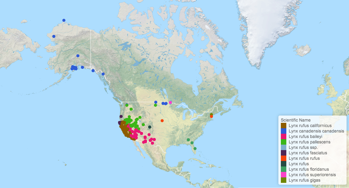
__Mapping observations__
The development version of the package includes a new function `ee_map()` that allows users to generate interactive maps from observation queries using Leaflet.js.
```r
lynx_data <- ee_observations(genus = "Lynx", georeferenced = TRUE, page = "all", quiet = TRUE)
ee_map(lynx_data)
```
### Photos
The ecoengine also contains a large number of photos from various sources. It's easy to query the photo database using similar arguments as above. One can search by taxa, location, source, collection and much more.
```r
photos <- ee_photos(quiet = TRUE, progress = FALSE)
photos
```
```
## [Total results on the server]: 72454
## [Args]:
## page_size = 1000
## georeferenced = 0
## page = 1
## [Type]: photos
## [Number of results retrieved]: 1000
```
The database currently holds 72454 photos. Photos can be searched by state province, county, genus, scientific name, authors along with date bounds. For additional options see `?ee_photos`.
#### Searching photos by author
```r
charles_results <- ee_photos(author = "Charles Webber", quiet = TRUE, progress = FALSE)
charles_results
```
```
## [Total results on the server]: 4907
## [Args]:
## page_size = 1000
## authors = Charles Webber
## georeferenced = FALSE
## page = 1
## [Type]: photos
## [Number of results retrieved]: 1000
```
```r
# Let's examine a couple of rows of the data
charles_results$data[1:2, ]
```
```
## url
## 1 https://ecoengine.berkeley.edu/api/photos/CalPhotos%3A8076%2B3101%2B2933%2B0025/
## 2 https://ecoengine.berkeley.edu/api/photos/CalPhotos%3A8076%2B3101%2B0667%2B0107/
## record authors
## 1 CalPhotos:8076+3101+2933+0025 Charles Webber
## 2 CalPhotos:8076+3101+0667+0107 Charles Webber
## locality county photog_notes
## 1 Yosemite National Park, Badger Pass Mariposa County Tan Oak
## 2 Yosemite National Park, Yosemite Falls Mariposa County
## begin_date end_date collection_code scientific_name
## 1 CalAcademy Notholithocarpus densiflorus
## 2 CalAcademy Rhododendron occidentale
## url
## 1 https://ecoengine.berkeley.edu/api/observations/CalPhotos%3A8076%2B3101%2B2933%2B0025%3A1/
## 2 https://ecoengine.berkeley.edu/api/observations/CalPhotos%3A8076%2B3101%2B0667%2B0107%3A1/
## license
## 1 CC BY-NC-SA 3.0
## 2 CC BY-NC-SA 3.0
## media_url
## 1 http://calphotos.berkeley.edu/imgs/512x768/8076_3101/2933/0025.jpeg
## 2 http://calphotos.berkeley.edu/imgs/512x768/8076_3101/0667/0107.jpeg
## remote_resource
## 1 http://calphotos.berkeley.edu/cgi/img_query?seq_num=21272&one=T
## 2 http://calphotos.berkeley.edu/cgi/img_query?seq_num=14468&one=T
## source geojson.type longitude
## 1 https://ecoengine.berkeley.edu/api/sources/9/ Point -119.657387
## 2 https://ecoengine.berkeley.edu/api/sources/9/ Point -119.597389
## latitude
## 1 37.663724
## 2 37.753851
```
---
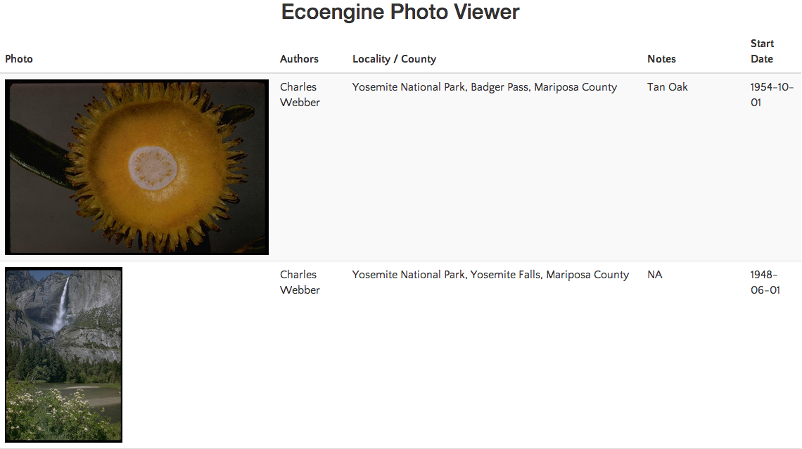
#### Browsing these photos
```r
view_photos(charles_results)
```
This will launch your default browser and render a page with thumbnails of all images returned by the search query. You can do this with any `ecoengine` object of type `photos`. Suggestions for improving the photo browser are welcome.
Other photo search examples
```r
# All the photos in the CDGA collection
all_cdfa <- ee_photos(collection_code = "CDFA", page = "all", progress = FALSE)
# All Racoon pictures
racoons <- ee_photos(scientific_name = "Procyon lotor", quiet = TRUE, progress = FALSE)
```
---
### Species checklists
There is a wealth of checklists from all the source locations. To get all available checklists from the engine, run:
```r
all_lists <- ee_checklists()
```
```
## Returning 52 checklists
```
```r
head(all_lists[, c("footprint", "subject")])
```
```
## footprint
## 1 https://ecoengine.berkeley.edu/api/footprints/angelo-reserve/
## 2 https://ecoengine.berkeley.edu/api/footprints/angelo-reserve/
## 3 https://ecoengine.berkeley.edu/api/footprints/angelo-reserve/
## 4 https://ecoengine.berkeley.edu/api/footprints/hastings-reserve/
## 5 https://ecoengine.berkeley.edu/api/footprints/angelo-reserve/
## 6 https://ecoengine.berkeley.edu/api/footprints/hastings-reserve/
## subject
## 1 Mammals
## 2 Mosses
## 3 Beetles
## 4 Spiders
## 5 Amphibians
## 6 Ants
```
Currently there are 52 lists available. We can drill deeper into any list to get all the available data. We can also narrow our checklist search to groups of interest (see `unique(all_lists$subject)`). For example, to get the list of Spiders:
```r
spiders <- ee_checklists(subject = "Spiders")
```
```
## Returning 1 checklists
```
```r
spiders
```
```
## record
## 4 bigcb:specieslist:15
## footprint
## 4 https://ecoengine.berkeley.edu/api/footprints/hastings-reserve/
## url
## 4 https://ecoengine.berkeley.edu/api/checklists/bigcb%3Aspecieslist%3A15/
## source subject
## 4 https://ecoengine.berkeley.edu/api/sources/18/ Spiders
```
Now we can drill deep into each list. For this tutorial I'll just retrieve data from the the two lists returned above.
```r
library(plyr)
spider_details <- ldply(spiders$url, checklist_details)
names(spider_details)
```
```
## [1] "url" "observation_type"
## [3] "scientific_name" "collection_code"
## [5] "institution_code" "country"
## [7] "state_province" "county"
## [9] "locality" "begin_date"
## [11] "end_date" "kingdom"
## [13] "phylum" "clss"
## [15] "order" "family"
## [17] "genus" "specific_epithet"
## [19] "infraspecific_epithet" "source"
## [21] "remote_resource" "earliest_period_or_lowest_system"
## [23] "latest_period_or_highest_system"
```
```r
unique(spider_details$scientific_name)
```
```
## [1] "Holocnemus pluchei" "Oecobius navus"
## [3] "Uloborus diversus" "Neriene litigiosa"
## [5] "Theridion " "Tidarren "
## [7] "Dictyna " "Mallos "
## [9] "Yorima " "Hahnia sanjuanensis"
## [11] "Cybaeus " "Zanomys "
## [13] "Anachemmis " "Titiotus "
## [15] "Oxyopes scalaris" "Zora hespera"
## [17] "Drassinella " "Phrurotimpus mateonus"
## [19] "Scotinella " "Castianeira luctifera"
## [21] "Meriola californica" "Drassyllus insularis"
## [23] "Herpyllus propinquus" "Micaria utahna"
## [25] "Trachyzelotes lyonneti" "Ebo evansae"
## [27] "Habronattus oregonensis" "Metaphidippus "
## [29] "Platycryptus californicus" "Calymmaria "
## [31] "Frontinella communis" "Undetermined "
## [33] "Latrodectus hesperus"
```
Our resulting dataset now contains 33 unique spider species.
### Searching the engine
The search is elastic by default. One can search for any field in `ee_observations()` across all available resources. For example,
```r
# The search function runs an automatic elastic search across all resources available through the engine.
lynx_results <- ee_search(query = "genus:Lynx")
lynx_results[, -3]
# This gives you a breakdown of what's available allowing you dig deeper.
```
```
## field results
## state_province.2 California 282
## state_province.21 Nevada 70
## state_province.3 Alaska 51
## state_province.4 British Columbia 34
## state_province.5 Arizona 24
## state_province.6 Montana 14
## state_province.7 Baja California Sur 13
## state_province.8 Baja California 12
## state_province.9 Zacatecas 10
## state_province.10 New Mexico 8
## kingdom animalia 562
## genus lynx 578
## resource Observations 578
## family felidae 563
## scientific_name.2 Lynx rufus californicus 232
## scientific_name.21 Lynx rufus baileyi 93
## scientific_name.3 Lynx canadensis canadensis 93
## scientific_name.4 Lynx rufus pallescens 76
## scientific_name.5 Lynx rufus 16
## scientific_name.6 Lynx rufus peninsularis 15
## scientific_name.7 Lynx canadensis 13
## scientific_name.8 Lynx rufus rufus 11
## scientific_name.9 Lynx rufus fasciatus 11
## scientific_name.10 Lynx rufus escuinapae 10
## country.2 United States 495
## country.21 Mexico 45
## country.3 Canada 34
## country.4 None 4
## clss mammalia 562
## order carnivora 561
## phylum chordata 559
## georeferenced.2 true 525
## georeferenced.21 false 53
## observation_type.2 specimen 557
## observation_type.21 photo 16
## observation_type.3 fossil 4
## observation_type.4 checklist 1
## decade.2 1931-1940 132
## decade.21 1921-1930 91
## decade.3 1911-1920 74
## decade.4 1901-1910 66
## decade.5 1971-1980 62
## decade.6 1941-1950 46
## decade.7 1961-1970 35
## decade.8 1951-1960 34
## decade.9 2001-2010 9
## decade.10 1991-2000 4
```
Similarly it's possible to search through the observations in a detailed manner as well.
```r
all_lynx_data <- ee_search_obs(query = "Lynx", page = "all", progress = FALSE)
```
```
## Search contains 644 observations (downloading 1 of 1 pages)
```
```r
all_lynx_data
```
```
## [Total results on the server]: 644
## [Args]:
## q = Lynx
## page_size = 1000
## page = all
## [Type]: observations
## [Number of results retrieved]: 644
```
---
### Miscellaneous functions
__Footprints__
`ee_footprints()` provides a list of all the footprints.
```r
footprints <- ee_footprints()
footprints[, -3] # To keep the table from spilling over
```
```
## name
## 1 Angelo Reserve
## 2 Sagehen Reserve
## 3 Hastings Reserve
## 4 Blue Oak Ranch Reserve
## url
## 1 https://ecoengine.berkeley.edu/api/footprints/angelo-reserve/
## 2 https://ecoengine.berkeley.edu/api/footprints/sagehen-reserve/
## 3 https://ecoengine.berkeley.edu/api/footprints/hastings-reserve/
## 4 https://ecoengine.berkeley.edu/api/footprints/blue-oak-ranch-reserve/
```
__Data sources__
`ee_sources()` provides a list of data sources for the specimens contained in the museum.
```r
source_list <- ee_sources()
unique(source_list$name)
```
```
## name
## 1 UCANR Drought images
## 2 LACM Vertebrate Collection
## 3 CAS Botany
## 4 CAS Entomology
## 5 MVZ Herp Collection
## 6 VTM plot coordinates
## 7 CAS Herpetology
## 8 VTM plot data
## 9 CAS Ornithology
## 10 Consortium of California Herbaria
```
To cite package `ecoengine` in publications use:
Karthik Ram (2014). ecoengine: Programmatic interface to the API
serving UC Berkeley's Natural History Data. R package version 1.3.
http://CRAN.R-project.org/package=ecoengine
A BibTeX entry for LaTeX users is
```
@Manual{,
title = {ecoengine: Programmatic interface to the API serving UC Berkeley's Natural
History Data},
author = {Karthik Ram},
year = {2014},
note = {R package version 1.9.2},
url = {http://CRAN.R-project.org/package=ecoengine},
}
```
## License and bugs
* License: [CC0](http://creativecommons.org/choose/zero/)
* Report bugs at [our Github repo for Ecoengine](https://github.com/ropensci/ecoengine/issues?state=open)
[Back to top](#top)
